Click here for setup information

knitr::opts_chunk$set(eval = FALSE, echo = TRUE)
set.seed(119)
#library(conflicted)
#pacman::p_depends(vegan, local = TRUE)  
#pacman::p_depends_reverse(vegan, local = TRUE)  
library(phyloseq); packageVersion("phyloseq")
pacman::p_load(ape, bestNormalize, tidyverse, gdata, mctoolsr, 
               ggpubr, ggvegan, ggfortify, vegan, reactable, 
               downloadthis, captioner, ggplot2,
               install = FALSE, update = FALSE)

options(scipen=999)
knitr::opts_current$get(c(
  "cache",
  "cache.path",
  "cache.rebuild",
  "dependson",
  "autodep"
))

Synopsis

In this workflow we compare the environmental metadata with the microbial community data. Part 1 involves the 16S rRNA community data and Part 2 deals with the ITS community data. Each workflow contains the same major steps:

Metadata Normality Tests: Shapiro-Wilk Normality Test to test whether each matadata parameter is normally distributed.
Normalize Parameters: R package bestNormalize to find and execute the best normalizing transformation.
Split Metadata parameters into groups: a) Environmental and edaphic properties, b) Microbial functional responses, and c) Temperature adaptation properties.
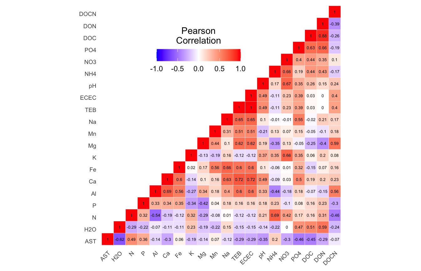
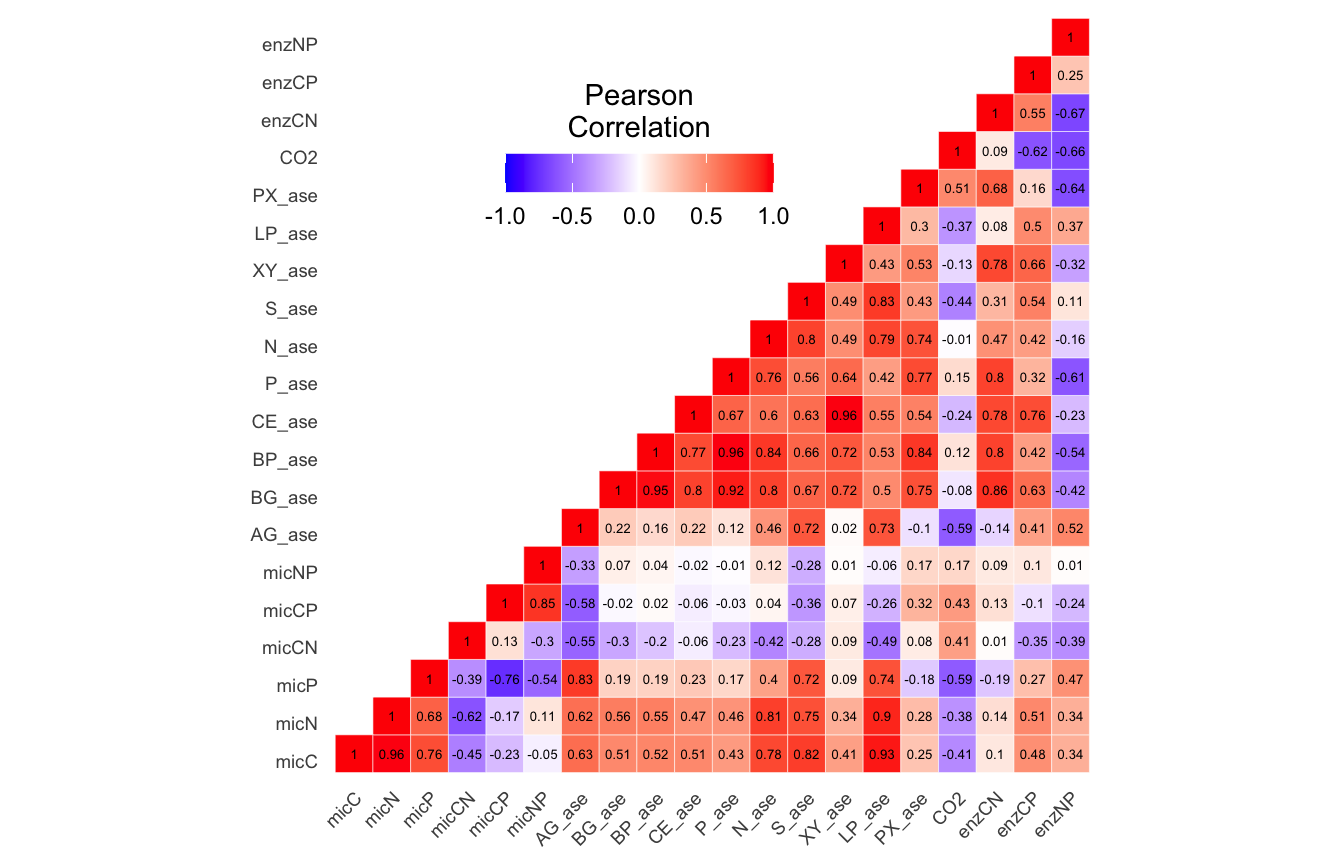
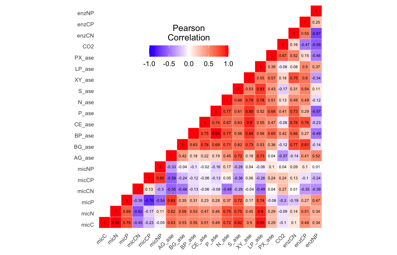
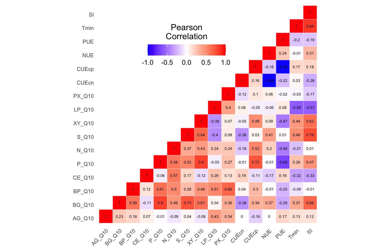
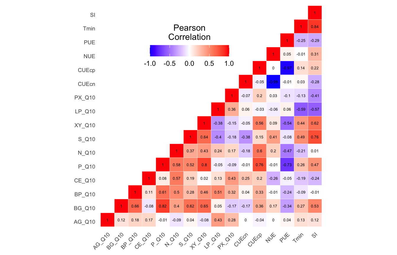
Autocorrelation Tests: Test all possible pair-wise comparisons, on both normalized and non-normalized data sets, for each group.
Remove autocorrelated parameters from each group.
Dissimilarity Correlation Tests: Use Mantel Tests to see if any on the metadata groups are significantly correlated with the community data.
Best Subset of Variables: Determine which of the metadata parameters from each group are the most strongly correlated with the community data. For this we use the bioenv function from the vegan (Oksanen et al. 2012) package.
Distance-based Redundancy Analysis: Ordination analysis of samples and metadata vector overlays using capscale, also from the vegan package.

Workflow Input

Files needed to run this workflow can be downloaded from figshare. You will also need the metadata table, which can be accessed below.

Metadata

In this section we provide access to the complete environmental metadata containing 61 parameters across all 15 samples.

(common) Table 1 | Metadata values for each sample.

Multivariate Summary

Summary results for of envfit and bioenv tests for edaphic properties, soil functional response, and temperature adaptation for both 16S rRNA and ITS data sets.

16S rRNA

Metadata parameters removed based on autocorrelation results.

edaphic properties: TEB + DON + Na + Al + Ca
soil functional response: micN + micNP + enzCN + enzCP + BP_ase + CE_ase + LP_ase + N_ase + P_ase
temperature adaptation: NUE + PUE + SI

Metadata parameters removed from capscale analysis based on Degrees of Freedom.

edaphic properties: Mg + Mn
soil functional response: NONE
temperature adaptation: NONE

(16S rRNA) Table 1 | Significant results of envfit & bioenv tests for the 16S rRNA data set.

ITS

Metadata parameters removed based on autocorrelation results.

edaphic properties: TEB + DON + Na + Al + Ca
soil functional response: micN + micNP + enzCN + enzCP + BP_ase + CE_ase + LP_ase + N_ase + P_ase
temperature adaptation: NUE + PUE + P_Q10 + SI

Metadata parameters removed from capscale analysis based on Degrees of Freedom.

edaphic properties: Mg + Mn + Na + Al + Fe + K
soil functional response: NONE
temperature adaptation: S_Q10

(ITS) Table 1 | Significant results of envfit & bioenv tests for the ITS data set.

16s rRNA

Data Formating

Transform ps Objects

The first step is to transform the phyloseq objects.

Show the code

samp_ps <- c("ssu18_ps_work", "ssu18_ps_pime", "ssu18_ps_perfect", 
             "ssu18_ps_work_otu", "ssu18_ps_pime_otu", "ssu18_ps_perfect_otu")
for (i in samp_ps) {
     tmp_get <- get(i)
     tmp_ps <- transform_sample_counts(tmp_get, function(otu) 1e5 * otu/sum(otu))
     tmp_ps@phy_tree <- NULL
     tmp_ps <- prune_samples(sample_sums(tmp_ps) > 0, tmp_ps)
     tmp_tree <- rtree(ntaxa(tmp_ps), rooted = TRUE, tip.label = taxa_names(tmp_ps))
     tmp_samp <- data.frame(sample_data(tmp_get))
     tmp_samp <- tmp_samp %>% dplyr::rename("TREAT_T" = "TEMP")
     tmp_ps <- merge_phyloseq(tmp_ps, sample_data, tmp_tree)
     sample_data(tmp_ps) <- tmp_samp
     tmp_name <- purrr::map_chr(i, ~ paste0(., "_prop"))
     print(tmp_name)
     assign(tmp_name, tmp_ps)
     rm(list = ls(pattern = "tmp_"))
}

Format for mctoolsr

Then a bit of formatting to make the data compatible with mctoolsr.

Show the code

for (i in samp_ps) {
     tmp_get <- get(purrr::map_chr(i, ~ paste0(., "_prop")))
     tmp_tax <- data.frame(tax_table(tmp_get))
     tmp_tax$ASV_SEQ <- NULL
     
     tmp_col_names <- colnames(tmp_tax)
     tmp_tax_merge <- tmp_tax %>% tidyr::unite(taxonomy, 
                                               all_of(tmp_col_names), 
                                               sep = ";")
     tmp_tax_merge <- tmp_tax_merge %>% tibble::rownames_to_column("#OTU_ID")
     tmp_otu <- data.frame(t(otu_table(tmp_get)))
     tmp_otu <- tmp_otu %>% tibble::rownames_to_column("#OTU_ID")
     tmp_otu_tax <- dplyr::left_join(tmp_otu, tmp_tax_merge, by = "#OTU_ID")

     tmp_samp <- data.frame(sample_data(tmp_get))
     tmp_samp[,c(1,3)] <- NULL
     tmp_samp <- tmp_samp %>% tibble::rownames_to_column("#SampleID")

     tmp_metad <- metad %>% dplyr::rename("#SampleID" = "id")
     tmp_metad[,2:5] <- NULL
     tmp_md <- dplyr::left_join(tmp_samp, tmp_metad, by = "#SampleID")
     
     tmp_otu_name <- purrr::map_chr(i, ~ paste0(., "_otu_tax"))
     print(tmp_otu_name)
     assign(tmp_otu_name, tmp_otu_tax)

     tmp_md_name <- purrr::map_chr(i, ~ paste0(., "_md"))
     print(tmp_md_name)
     assign(tmp_md_name, tmp_md)

     tmp_path <- file.path("files/metadata/tables/")
     write_delim(tmp_otu_tax, paste(tmp_path, tmp_otu_name, ".txt", sep = ""), delim = "\t")
     write_delim(tmp_md, paste(tmp_path, tmp_md_name, ".txt", sep = ""), delim = "\t")
     rm(list = ls(pattern = "tmp_"))
}

Show the code

for (i in samp_ps) {
     tmp_path <- file.path("files/metadata/tables/")
     tmp_otu_name <- purrr::map_chr(i, ~ paste0(., "_otu_tax"))
     tmp_md_name <- purrr::map_chr(i, ~ paste0(., "_md"))
     tmp_tax_table_fp <- paste(tmp_path, tmp_otu_name, ".txt", sep = "")
     tmp_map_fp <- paste(tmp_path, tmp_md_name, ".txt", sep = "")
     tmp_input <- load_taxa_table(tmp_tax_table_fp, tmp_map_fp)
     tmp_input_name <- purrr::map_chr(i, ~ paste0(., "_mc"))
     print(tmp_input_name)
     assign(tmp_input_name, tmp_input)
     rm(list = ls(pattern = "tmp_"))
}
rm(list = ls(pattern = "_md"))
rm(list = ls(pattern = "_otu_tax"))

Choose Data Set

At this point in the code we need to choose a data set to use, formatted with mctoolsr. Remember, there are four choices:

FULL, unfiltered data set.
Arbitrary filtered data set.
PERfect filtered data set.
PIME filtered data set.

This way, if we want to test other data sets we only need to change the name here.

objects(pattern = "_mc")
ssu18_select_mc <- ssu18_ps_pime_mc

Normality Tests

Before proceeding, we need to test each parameter in the metadata to see which ones are and are not normally distributed. For that, we use the Shapiro-Wilk Normality Test. Here we only need one of the metadata files.

Show the code

temp_md <- ssu18_select_mc$map_loaded
temp_md[,1:9] <- NULL
shap_results <- NULL

for (i in colnames(temp_md)) {
  tmp_shap <- shapiro.test(temp_md[[i]])
  tmp_p <- round(tmp_shap$p.value, digits = 5)
  tmp_res <- eval(isTRUE(tmp_shap$p.value < 0.05))
  shap_results <- rbind(shap_results, data.frame(i, tmp_p, tmp_res))
  rm(list = ls(pattern = "tmp_"))
}
colnames(shap_results) <- c("parameter", "p-value", "tranform")
shap_results
dplyr::filter(shap_results, tranform == "TRUE")
md_to_tranform <- shap_results$parameter[shap_results$tranform == TRUE]
rm(list = ls(pattern = "temp_md"))

Show the results of each normality test for metadata parameters

(16S rRNA) Table 2 | Results of the Shapiro-Wilk Normality Tests. P-values in red are significance (p-value < 0.05) meaning the parameter needs to be normalized.

Looks like we need to transform 25 metadata parameters.

Normalize Parameters

Here we use the R package bestNormalize to find and execute the best normalizing transformation. The function will test the following normalizing transformations:

arcsinh_x performs an arcsinh transformation.
boxcox Perform a Box-Cox transformation and center/scale a vector to attempt normalization. boxcox estimates the optimal value of lambda for the Box-Cox transformation. The function will return an error if a user attempt to transform nonpositive data.
yeojohnson Perform a Yeo-Johnson Transformation and center/scale a vector to attempt normalization. yeojohnson estimates the optimal value of lambda for the Yeo-Johnson transformation. The Yeo-Johnson is similar to the Box-Cox method, however it allows for the transformation of nonpositive data as well.
orderNorm The Ordered Quantile (ORQ) normalization transformation, orderNorm(), is a rank-based procedure by which the values of a vector are mapped to their percentile, which is then mapped to the same percentile of the normal distribution. Without the presence of ties, this essentially guarantees that the transformation leads to a uniform distribution.
log_x performs a simple log transformation. The parameter a is essentially estimated by the training set by default (estimated as the minimum possible to some extent epsilon), while the base must be specified beforehand. The default base of the log is 10.
sqrt_x performs a simple square-root transformation. The parameter a is essentially estimated by the training set by default (estimated as the minimum possible), while the base must be specified beforehand.
exp_x performs a simple exponential transformation.

See this GitHub issue (#5) for a description on getting reproducible results. Apparently, you can get different results because the bestNormalize() function uses repeated cross-validation (and doesn’t automatically set the seed), so the results will be slightly different each time the function is executed.

Show the code

set.seed(119)
for (i in md_to_tranform) {
  tmp_md <- ssu18_select_mc$map_loaded
  tmp_best_norm <- bestNormalize(tmp_md[[i]], r = 1, k = 5, loo = TRUE)
  tmp_name <- purrr::map_chr(i, ~ paste0(., "_best_norm_test"))
  assign(tmp_name, tmp_best_norm)
  print(tmp_name)
  rm(list = ls(pattern = "tmp_"))
}

Show the chosen transformations


## bestNormalize Chosen transformation of AST ## 
orderNorm Transformation with 15 nonmissing obs and no ties 
 - Original quantiles:
    0%    25%    50%    75%   100% 
25.800 26.275 28.800 30.280 41.770 
_____________________________________

## bestNormalize Chosen transformation of H2O ## 
orderNorm Transformation with 15 nonmissing obs and no ties 
 - Original quantiles:
   0%   25%   50%   75%  100% 
0.204 0.308 0.370 0.384 0.401 
_____________________________________

## bestNormalize Chosen transformation of Al ## 
Standardized asinh(x) Transformation with 15 nonmissing obs.:
 Relevant statistics:
 - mean (before standardization) = 0.0059997 
 - sd (before standardization) = 0.008280287 
_____________________________________

## bestNormalize Chosen transformation of Ca ## 
orderNorm Transformation with 15 nonmissing obs and ties
 - 10 unique values 
 - Original quantiles:
   0%   25%   50%   75%  100% 
25.49 27.19 29.23 34.36 39.79 
_____________________________________

## bestNormalize Chosen transformation of Fe ## 
Standardized asinh(x) Transformation with 15 nonmissing obs.:
 Relevant statistics:
 - mean (before standardization) = 0.0119984 
 - sd (before standardization) = 0.01264569 
_____________________________________

## bestNormalize Chosen transformation of TEB ## 
orderNorm Transformation with 15 nonmissing obs and ties
 - 10 unique values 
 - Original quantiles:
  0%  25%  50%  75% 100% 
41.6 43.3 45.1 51.4 61.7 
_____________________________________

## bestNormalize Chosen transformation of ECEC ## 
orderNorm Transformation with 15 nonmissing obs and ties
 - 10 unique values 
 - Original quantiles:
  0%  25%  50%  75% 100% 
41.7 43.3 45.3 51.5 61.8 
_____________________________________

## bestNormalize Chosen transformation of minNO3 ## 
Standardized Box Cox Transformation with 15 nonmissing obs.:
 Estimated statistics:
 - lambda = -0.3344538 
 - mean (before standardization) = 1.907818 
 - sd (before standardization) = 0.2388776 
_____________________________________

## bestNormalize Chosen transformation of minTIN ## 
orderNorm Transformation with 15 nonmissing obs and ties
 - 14 unique values 
 - Original quantiles:
     0%     25%     50%     75%    100% 
  8.760  14.995  23.080  39.935 110.750 
_____________________________________

## bestNormalize Chosen transformation of DOC ## 
orderNorm Transformation with 15 nonmissing obs and no ties 
 - Original quantiles:
     0%     25%     50%     75%    100% 
 30.800  44.070  56.680  64.385 118.740 
_____________________________________

## bestNormalize Chosen transformation of DOCN ## 
orderNorm Transformation with 15 nonmissing obs and no ties 
 - Original quantiles:
    0%    25%    50%    75%   100% 
 9.440 10.290 11.150 12.095 19.270 
_____________________________________

## bestNormalize Chosen transformation of micCN ## 
orderNorm Transformation with 15 nonmissing obs and ties
 - 14 unique values 
 - Original quantiles:
   0%   25%   50%   75%  100% 
4.420 4.585 4.720 5.415 5.850 
_____________________________________

## bestNormalize Chosen transformation of BG_ase ## 
orderNorm Transformation with 15 nonmissing obs and no ties 
 - Original quantiles:
    0%    25%    50%    75%   100% 
 3.010  3.735  4.220  5.795 10.480 
_____________________________________

## bestNormalize Chosen transformation of BP_ase ## 
Standardized Log_b(x + a) Transformation with 15 nonmissing obs.:
 Relevant statistics:
 - a = 0 
 - b = 10 
 - mean (before standardization) = 0.5217757 
 - sd (before standardization) = 0.2001498 
_____________________________________

## bestNormalize Chosen transformation of CE_ase ## 
Standardized Log_b(x + a) Transformation with 15 nonmissing obs.:
 Relevant statistics:
 - a = 0 
 - b = 10 
 - mean (before standardization) = 0.03306978 
 - sd (before standardization) = 0.1652591 
_____________________________________

## bestNormalize Chosen transformation of P_ase ## 
orderNorm Transformation with 15 nonmissing obs and no ties 
 - Original quantiles:
    0%    25%    50%    75%   100% 
13.020 15.130 19.210 24.455 44.040 
_____________________________________

## bestNormalize Chosen transformation of N_ase ## 
orderNorm Transformation with 15 nonmissing obs and no ties 
 - Original quantiles:
  0%  25%  50%  75% 100% 
2.57 2.93 3.58 5.04 9.43 
_____________________________________

## bestNormalize Chosen transformation of XY_ase ## 
orderNorm Transformation with 15 nonmissing obs and ties
 - 13 unique values 
 - Original quantiles:
  0%  25%  50%  75% 100% 
0.66 0.81 1.11 1.39 2.52 
_____________________________________

## bestNormalize Chosen transformation of BG_Q10 ## 
orderNorm Transformation with 15 nonmissing obs and ties
 - 13 unique values 
 - Original quantiles:
   0%   25%   50%   75%  100% 
1.310 1.360 1.390 1.545 1.760 
_____________________________________

## bestNormalize Chosen transformation of BP_Q10 ## 
orderNorm Transformation with 15 nonmissing obs and ties
 - 11 unique values 
 - Original quantiles:
   0%   25%   50%   75%  100% 
1.340 1.415 1.440 1.530 1.740 
_____________________________________

## bestNormalize Chosen transformation of CO2 ## 
orderNorm Transformation with 15 nonmissing obs and ties
 - 14 unique values 
 - Original quantiles:
    0%    25%    50%    75%   100% 
 2.080  4.370  5.270 10.585 40.470 
_____________________________________

## bestNormalize Chosen transformation of PX_ase ## 
orderNorm Transformation with 15 nonmissing obs and no ties 
 - Original quantiles:
     0%     25%     50%     75%    100% 
 81.250  95.565 119.750 218.370 339.600 
_____________________________________

## bestNormalize Chosen transformation of PX_Q10 ## 
Standardized Yeo-Johnson Transformation with 15 nonmissing obs.:
 Estimated statistics:
 - lambda = -4.999946 
 - mean (before standardization) = 0.1968247 
 - sd (before standardization) = 0.001294011 
_____________________________________

## bestNormalize Chosen transformation of CUEcp ## 
Standardized Box Cox Transformation with 15 nonmissing obs.:
 Estimated statistics:
 - lambda = -0.9999576 
 - mean (before standardization) = -4.229896 
 - sd (before standardization) = 0.9115063 
_____________________________________

## bestNormalize Chosen transformation of PUE ## 
orderNorm Transformation with 15 nonmissing obs and ties
 - 7 unique values 
 - Original quantiles:
   0%   25%   50%   75%  100% 
0.770 0.880 0.900 0.905 0.920 
_____________________________________

Show the complete bestNormalize results


## Results of bestNormalize for AST ## 
Best Normalizing transformation with 15 Observations
 Estimated Normality Statistics (Pearson P / df, lower => more normal):
 - arcsinh(x): 3.4
 - Box-Cox: 1.8
 - Center+scale: 4.2
 - Exp(x): 21.2667
 - Log_b(x+a): 3.4
 - orderNorm (ORQ): 0.2
 - sqrt(x + a): 4.2
 - Yeo-Johnson: 2.8667
Estimation method: Out-of-sample via leave-one-out CV
 
Based off these, bestNormalize chose:
orderNorm Transformation with 15 nonmissing obs and no ties 
 - Original quantiles:
    0%    25%    50%    75%   100% 
25.800 26.275 28.800 30.280 41.770 
_____________________________________

## Results of bestNormalize for H2O ## 
Best Normalizing transformation with 15 Observations
 Estimated Normality Statistics (Pearson P / df, lower => more normal):
 - arcsinh(x): 6.8667
 - Box-Cox: 5.8
 - Center+scale: 5.8
 - Exp(x): 5.8
 - Log_b(x+a): 6.0667
 - orderNorm (ORQ): 0.7333
 - sqrt(x + a): 6.8667
 - Yeo-Johnson: 5.8
Estimation method: Out-of-sample via leave-one-out CV
 
Based off these, bestNormalize chose:
orderNorm Transformation with 15 nonmissing obs and no ties 
 - Original quantiles:
   0%   25%   50%   75%  100% 
0.204 0.308 0.370 0.384 0.401 
_____________________________________

## Results of bestNormalize for Al ## 
Best Normalizing transformation with 15 Observations
 Estimated Normality Statistics (Pearson P / df, lower => more normal):
 - arcsinh(x): 8.2
 - Center+scale: 8.2
 - Exp(x): 8.2
 - Log_b(x+a): 8.2
 - orderNorm (ORQ): 8.2
 - sqrt(x + a): 8.2
 - Yeo-Johnson: 8.2
Estimation method: Out-of-sample via leave-one-out CV
 
Based off these, bestNormalize chose:
Standardized asinh(x) Transformation with 15 nonmissing obs.:
 Relevant statistics:
 - mean (before standardization) = 0.0059997 
 - sd (before standardization) = 0.008280287 
_____________________________________

## Results of bestNormalize for Ca ## 
Best Normalizing transformation with 15 Observations
 Estimated Normality Statistics (Pearson P / df, lower => more normal):
 - arcsinh(x): 1.8
 - Box-Cox: 1.8
 - Center+scale: 3.4
 - Exp(x): 18.0667
 - Log_b(x+a): 1.8
 - orderNorm (ORQ): 0.2
 - sqrt(x + a): 1.8
 - Yeo-Johnson: 1.2667
Estimation method: Out-of-sample via leave-one-out CV
 
Based off these, bestNormalize chose:
orderNorm Transformation with 15 nonmissing obs and ties
 - 10 unique values 
 - Original quantiles:
   0%   25%   50%   75%  100% 
25.49 27.19 29.23 34.36 39.79 
_____________________________________

## Results of bestNormalize for Fe ## 
Best Normalizing transformation with 15 Observations
 Estimated Normality Statistics (Pearson P / df, lower => more normal):
 - arcsinh(x): 6.3333
 - Center+scale: 6.3333
 - Exp(x): 6.3333
 - Log_b(x+a): 6.3333
 - orderNorm (ORQ): 6.3333
 - sqrt(x + a): 6.3333
 - Yeo-Johnson: 6.3333
Estimation method: Out-of-sample via leave-one-out CV
 
Based off these, bestNormalize chose:
Standardized asinh(x) Transformation with 15 nonmissing obs.:
 Relevant statistics:
 - mean (before standardization) = 0.0119984 
 - sd (before standardization) = 0.01264569 
_____________________________________

## Results of bestNormalize for TEB ## 
Best Normalizing transformation with 15 Observations
 Estimated Normality Statistics (Pearson P / df, lower => more normal):
 - arcsinh(x): 2.3333
 - Box-Cox: 1.2667
 - Center+scale: 6.0667
 - Exp(x): 18.0667
 - Log_b(x+a): 2.3333
 - orderNorm (ORQ): 0.4667
 - sqrt(x + a): 5.5333
 - Yeo-Johnson: 1.5333
Estimation method: Out-of-sample via leave-one-out CV
 
Based off these, bestNormalize chose:
orderNorm Transformation with 15 nonmissing obs and ties
 - 10 unique values 
 - Original quantiles:
  0%  25%  50%  75% 100% 
41.6 43.3 45.1 51.4 61.7 
_____________________________________

## Results of bestNormalize for ECEC ## 
Best Normalizing transformation with 15 Observations
 Estimated Normality Statistics (Pearson P / df, lower => more normal):
 - arcsinh(x): 1.2667
 - Box-Cox: 1.2667
 - Center+scale: 6.0667
 - Exp(x): 18.0667
 - Log_b(x+a): 1.2667
 - orderNorm (ORQ): 0.4667
 - sqrt(x + a): 3.9333
 - Yeo-Johnson: 1.5333
Estimation method: Out-of-sample via leave-one-out CV
 
Based off these, bestNormalize chose:
orderNorm Transformation with 15 nonmissing obs and ties
 - 10 unique values 
 - Original quantiles:
  0%  25%  50%  75% 100% 
41.7 43.3 45.3 51.5 61.8 
_____________________________________

## Results of bestNormalize for minNO3 ## 
Best Normalizing transformation with 15 Observations
 Estimated Normality Statistics (Pearson P / df, lower => more normal):
 - arcsinh(x): 1.8
 - Box-Cox: 1.2667
 - Center+scale: 3.9333
 - Exp(x): 21.2667
 - Log_b(x+a): 1.8
 - orderNorm (ORQ): 1.2667
 - sqrt(x + a): 1.8
 - Yeo-Johnson: 1.2667
Estimation method: Out-of-sample via leave-one-out CV
 
Based off these, bestNormalize chose:
Standardized Box Cox Transformation with 15 nonmissing obs.:
 Estimated statistics:
 - lambda = -0.3344538 
 - mean (before standardization) = 1.907818 
 - sd (before standardization) = 0.2388776 
_____________________________________

## Results of bestNormalize for minTIN ## 
Best Normalizing transformation with 15 Observations
 Estimated Normality Statistics (Pearson P / df, lower => more normal):
 - arcsinh(x): 1.8
 - Box-Cox: 1.8
 - Center+scale: 3.9333
 - Exp(x): 21.2667
 - Log_b(x+a): 1.8
 - orderNorm (ORQ): 0.7333
 - sqrt(x + a): 1.8
 - Yeo-Johnson: 1.8
Estimation method: Out-of-sample via leave-one-out CV
 
Based off these, bestNormalize chose:
orderNorm Transformation with 15 nonmissing obs and ties
 - 14 unique values 
 - Original quantiles:
     0%     25%     50%     75%    100% 
  8.760  14.995  23.080  39.935 110.750 
_____________________________________

## Results of bestNormalize for DOC ## 
Best Normalizing transformation with 15 Observations
 Estimated Normality Statistics (Pearson P / df, lower => more normal):
 - arcsinh(x): 2.3333
 - Box-Cox: 1.2667
 - Center+scale: 2.8667
 - Exp(x): 21.2667
 - Log_b(x+a): 2.3333
 - orderNorm (ORQ): 0.4667
 - sqrt(x + a): 2.8667
 - Yeo-Johnson: 1.2667
Estimation method: Out-of-sample via leave-one-out CV
 
Based off these, bestNormalize chose:
orderNorm Transformation with 15 nonmissing obs and no ties 
 - Original quantiles:
     0%     25%     50%     75%    100% 
 30.800  44.070  56.680  64.385 118.740 
_____________________________________

## Results of bestNormalize for DOCN ## 
Best Normalizing transformation with 15 Observations
 Estimated Normality Statistics (Pearson P / df, lower => more normal):
 - arcsinh(x): 2.3333
 - Box-Cox: 0.7333
 - Center+scale: 3.9333
 - Exp(x): 21.2667
 - Log_b(x+a): 2.3333
 - orderNorm (ORQ): 0.2
 - sqrt(x + a): 3.1333
 - Yeo-Johnson: 0.2
Estimation method: Out-of-sample via leave-one-out CV
 
Based off these, bestNormalize chose:
orderNorm Transformation with 15 nonmissing obs and no ties 
 - Original quantiles:
    0%    25%    50%    75%   100% 
 9.440 10.290 11.150 12.095 19.270 
_____________________________________

## Results of bestNormalize for micCN ## 
Best Normalizing transformation with 15 Observations
 Estimated Normality Statistics (Pearson P / df, lower => more normal):
 - arcsinh(x): 3.1333
 - Box-Cox: 3.1333
 - Center+scale: 3.1333
 - Exp(x): 5.5333
 - Log_b(x+a): 3.1333
 - orderNorm (ORQ): 0.2
 - sqrt(x + a): 3.1333
 - Yeo-Johnson: 3.1333
Estimation method: Out-of-sample via leave-one-out CV
 
Based off these, bestNormalize chose:
orderNorm Transformation with 15 nonmissing obs and ties
 - 14 unique values 
 - Original quantiles:
   0%   25%   50%   75%  100% 
4.420 4.585 4.720 5.415 5.850 
_____________________________________

## Results of bestNormalize for BG_ase ## 
Best Normalizing transformation with 15 Observations
 Estimated Normality Statistics (Pearson P / df, lower => more normal):
 - arcsinh(x): 2.8667
 - Box-Cox: 2.3333
 - Center+scale: 5
 - Exp(x): 21.2667
 - Log_b(x+a): 2.8667
 - orderNorm (ORQ): 0.4667
 - sqrt(x + a): 2.8667
 - Yeo-Johnson: 2.3333
Estimation method: Out-of-sample via leave-one-out CV
 
Based off these, bestNormalize chose:
orderNorm Transformation with 15 nonmissing obs and no ties 
 - Original quantiles:
    0%    25%    50%    75%   100% 
 3.010  3.735  4.220  5.795 10.480 
_____________________________________

## Results of bestNormalize for BP_ase ## 
Best Normalizing transformation with 15 Observations
 Estimated Normality Statistics (Pearson P / df, lower => more normal):
 - arcsinh(x): 1.5333
 - Box-Cox: 1.5333
 - Center+scale: 3.1333
 - Exp(x): 11.9333
 - Log_b(x+a): 0.7333
 - orderNorm (ORQ): 0.7333
 - sqrt(x + a): 3.1333
 - Yeo-Johnson: 1.5333
Estimation method: Out-of-sample via leave-one-out CV
 
Based off these, bestNormalize chose:
Standardized Log_b(x + a) Transformation with 15 nonmissing obs.:
 Relevant statistics:
 - a = 0 
 - b = 10 
 - mean (before standardization) = 0.5217757 
 - sd (before standardization) = 0.2001498 
_____________________________________

## Results of bestNormalize for CE_ase ## 
Best Normalizing transformation with 15 Observations
 Estimated Normality Statistics (Pearson P / df, lower => more normal):
 - arcsinh(x): 1
 - Box-Cox: 0.7333
 - Center+scale: 1.8
 - Exp(x): 4.2
 - Log_b(x+a): 0.4667
 - orderNorm (ORQ): 1
 - sqrt(x + a): 1
 - Yeo-Johnson: 0.4667
Estimation method: Out-of-sample via leave-one-out CV
 
Based off these, bestNormalize chose:
Standardized Log_b(x + a) Transformation with 15 nonmissing obs.:
 Relevant statistics:
 - a = 0 
 - b = 10 
 - mean (before standardization) = 0.03306978 
 - sd (before standardization) = 0.1652591 
_____________________________________

## Results of bestNormalize for P_ase ## 
Best Normalizing transformation with 15 Observations
 Estimated Normality Statistics (Pearson P / df, lower => more normal):
 - arcsinh(x): 2.0667
 - Box-Cox: 1.2667
 - Center+scale: 3.6667
 - Exp(x): 21.2667
 - Log_b(x+a): 2.0667
 - orderNorm (ORQ): 0.2
 - sqrt(x + a): 2.3333
 - Yeo-Johnson: 1.2667
Estimation method: Out-of-sample via leave-one-out CV
 
Based off these, bestNormalize chose:
orderNorm Transformation with 15 nonmissing obs and no ties 
 - Original quantiles:
    0%    25%    50%    75%   100% 
13.020 15.130 19.210 24.455 44.040 
_____________________________________

## Results of bestNormalize for N_ase ## 
Best Normalizing transformation with 15 Observations
 Estimated Normality Statistics (Pearson P / df, lower => more normal):
 - arcsinh(x): 1.2667
 - Box-Cox: 1.8
 - Center+scale: 3.1333
 - Exp(x): 17.8
 - Log_b(x+a): 1.2667
 - orderNorm (ORQ): 0.2
 - sqrt(x + a): 3.1333
 - Yeo-Johnson: 1.2667
Estimation method: Out-of-sample via leave-one-out CV
 
Based off these, bestNormalize chose:
orderNorm Transformation with 15 nonmissing obs and no ties 
 - Original quantiles:
  0%  25%  50%  75% 100% 
2.57 2.93 3.58 5.04 9.43 
_____________________________________

## Results of bestNormalize for XY_ase ## 
Best Normalizing transformation with 15 Observations
 Estimated Normality Statistics (Pearson P / df, lower => more normal):
 - arcsinh(x): 0.7333
 - Box-Cox: 0.7333
 - Center+scale: 2.8667
 - Exp(x): 6.3333
 - Log_b(x+a): 0.7333
 - orderNorm (ORQ): 0.2
 - sqrt(x + a): 1.8
 - Yeo-Johnson: 0.7333
Estimation method: Out-of-sample via leave-one-out CV
 
Based off these, bestNormalize chose:
orderNorm Transformation with 15 nonmissing obs and ties
 - 13 unique values 
 - Original quantiles:
  0%  25%  50%  75% 100% 
0.66 0.81 1.11 1.39 2.52 
_____________________________________

## Results of bestNormalize for BG_Q10 ## 
Best Normalizing transformation with 15 Observations
 Estimated Normality Statistics (Pearson P / df, lower => more normal):
 - arcsinh(x): 2.3333
 - Box-Cox: 2.3333
 - Center+scale: 2.3333
 - Exp(x): 6.0667
 - Log_b(x+a): 2.3333
 - orderNorm (ORQ): 0.2
 - sqrt(x + a): 2.3333
 - Yeo-Johnson: 2.3333
Estimation method: Out-of-sample via leave-one-out CV
 
Based off these, bestNormalize chose:
orderNorm Transformation with 15 nonmissing obs and ties
 - 13 unique values 
 - Original quantiles:
   0%   25%   50%   75%  100% 
1.310 1.360 1.390 1.545 1.760 
_____________________________________

## Results of bestNormalize for BP_Q10 ## 
Best Normalizing transformation with 15 Observations
 Estimated Normality Statistics (Pearson P / df, lower => more normal):
 - arcsinh(x): 2.6
 - Box-Cox: 2.6
 - Center+scale: 2.6
 - Exp(x): 2.6
 - Log_b(x+a): 2.6
 - orderNorm (ORQ): 0.7333
 - sqrt(x + a): 2.6
 - Yeo-Johnson: 2.3333
Estimation method: Out-of-sample via leave-one-out CV
 
Based off these, bestNormalize chose:
orderNorm Transformation with 15 nonmissing obs and ties
 - 11 unique values 
 - Original quantiles:
   0%   25%   50%   75%  100% 
1.340 1.415 1.440 1.530 1.740 
_____________________________________

## Results of bestNormalize for CO2 ## 
Best Normalizing transformation with 15 Observations
 Estimated Normality Statistics (Pearson P / df, lower => more normal):
 - arcsinh(x): 1.5333
 - Box-Cox: 2.6
 - Center+scale: 11.9333
 - Exp(x): 21.2667
 - Log_b(x+a): 1.5333
 - orderNorm (ORQ): 1.2667
 - sqrt(x + a): 3.4
 - Yeo-Johnson: 2.0667
Estimation method: Out-of-sample via leave-one-out CV
 
Based off these, bestNormalize chose:
orderNorm Transformation with 15 nonmissing obs and ties
 - 14 unique values 
 - Original quantiles:
    0%    25%    50%    75%   100% 
 2.080  4.370  5.270 10.585 40.470 
_____________________________________

## Results of bestNormalize for PX_ase ## 
Best Normalizing transformation with 15 Observations
 Estimated Normality Statistics (Pearson P / df, lower => more normal):
 - arcsinh(x): 2.3333
 - Box-Cox: 1.2667
 - Center+scale: 7.6667
 - Exp(x): 21.2667
 - Log_b(x+a): 2.3333
 - orderNorm (ORQ): 0.2
 - sqrt(x + a): 2.8667
 - Yeo-Johnson: 1.2667
Estimation method: Out-of-sample via leave-one-out CV
 
Based off these, bestNormalize chose:
orderNorm Transformation with 15 nonmissing obs and no ties 
 - Original quantiles:
     0%     25%     50%     75%    100% 
 81.250  95.565 119.750 218.370 339.600 
_____________________________________

## Results of bestNormalize for PX_Q10 ## 
Best Normalizing transformation with 15 Observations
 Estimated Normality Statistics (Pearson P / df, lower => more normal):
 - arcsinh(x): 14.6
 - Box-Cox: 4.2
 - Center+scale: 21.2667
 - Exp(x): 21.2667
 - Log_b(x+a): 11.9333
 - orderNorm (ORQ): 2.0667
 - sqrt(x + a): 21.2667
 - Yeo-Johnson: 1.5333
Estimation method: Out-of-sample via leave-one-out CV
 
Based off these, bestNormalize chose:
Standardized Yeo-Johnson Transformation with 15 nonmissing obs.:
 Estimated statistics:
 - lambda = -4.999946 
 - mean (before standardization) = 0.1968247 
 - sd (before standardization) = 0.001294011 
_____________________________________

## Results of bestNormalize for CUEcp ## 
Best Normalizing transformation with 15 Observations
 Estimated Normality Statistics (Pearson P / df, lower => more normal):
 - arcsinh(x): 3.9333
 - Box-Cox: 1.5333
 - Center+scale: 3.9333
 - Exp(x): 3.9333
 - Log_b(x+a): 2.0667
 - orderNorm (ORQ): 1.5333
 - sqrt(x + a): 2.0667
 - Yeo-Johnson: 2.0667
Estimation method: Out-of-sample via leave-one-out CV
 
Based off these, bestNormalize chose:
Standardized Box Cox Transformation with 15 nonmissing obs.:
 Estimated statistics:
 - lambda = -0.9999576 
 - mean (before standardization) = -4.229896 
 - sd (before standardization) = 0.9115063 
_____________________________________

## Results of bestNormalize for PUE ## 
Best Normalizing transformation with 15 Observations
 Estimated Normality Statistics (Pearson P / df, lower => more normal):
 - arcsinh(x): 8.2
 - Box-Cox: 9.8
 - Center+scale: 8.2
 - Exp(x): 3.9333
 - Log_b(x+a): 9.8
 - orderNorm (ORQ): 2.0667
 - sqrt(x + a): 9.8
 - Yeo-Johnson: 9.8
Estimation method: Out-of-sample via leave-one-out CV
 
Based off these, bestNormalize chose:
orderNorm Transformation with 15 nonmissing obs and ties
 - 7 unique values 
 - Original quantiles:
   0%   25%   50%   75%  100% 
0.770 0.880 0.900 0.905 0.920 
_____________________________________

Great, now we can add the normalized transformed data back to our mctoolsr metadata file.

Show the code

ssu18_select_mc_norm <- ssu18_select_mc

for (i in md_to_tranform) {
      tmp_get <- get(purrr::map_chr(i, ~ paste0(i, "_best_norm_test")))
      tmp_new_data <- tmp_get$x.t
      ssu18_select_mc_norm$map_loaded[[i]] <- tmp_new_data
      rm(list = ls(pattern = "tmp_"))
}

And rerun the Shapiro Tests.

Show the code

temp_md_norm <- ssu18_select_mc_norm$map_loaded
temp_md_norm[,1:9] <- NULL
shap_results_norm <- NULL

for (i in colnames(temp_md_norm)) {
  tmp_shap <- shapiro.test(temp_md_norm[[i]])
  tmp_p <- round(tmp_shap$p.value, digits = 5)
  tmp_res <- eval(isTRUE(tmp_shap$p.value < 0.05))
  shap_results_norm <- rbind(shap_results_norm, data.frame(i, tmp_p, tmp_res))
  rm(list = ls(pattern = "tmp_"))
}
colnames(shap_results_norm) <- c("parameter", "p-value", "tranform")
shap_results_norm
rm(list = ls(pattern = "temp_md_norm"))

And check if there are any parameters that are still significant for the normality test.

shap_results$parameter[shap_results_norm$tranform == TRUE]

[1] "Al" "Fe"

Ok. Looks like bestNormalize was unable to find a suitable transformation for Al and Fe. This is likely because there is very little variation in these metadata and/or there are too few significant digits.

Normalized Metadata

Finally, here is a new summary table that includes all of the normalized data.

(16S rRNA) Table 3 | Results of bestNormalize function applied to each parameter.

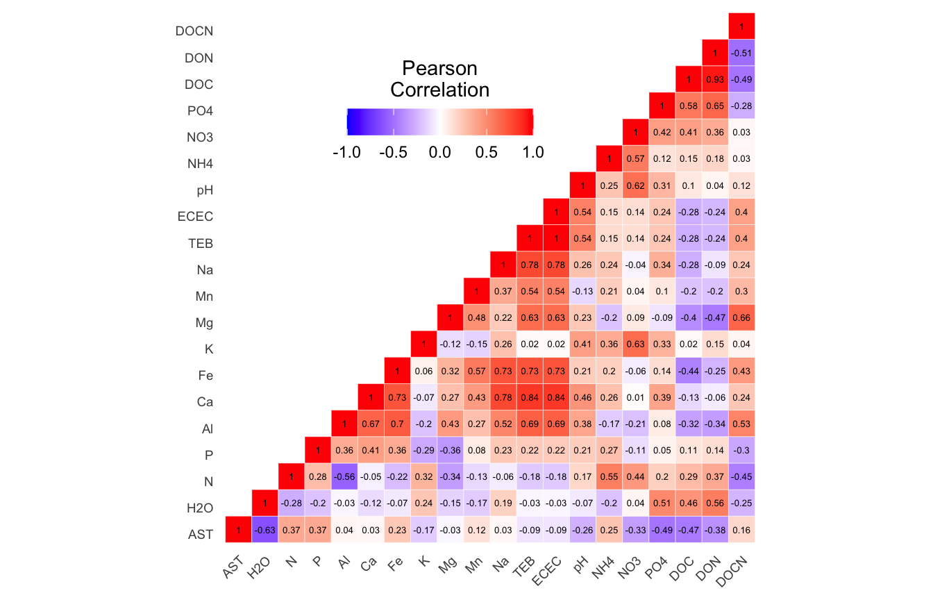
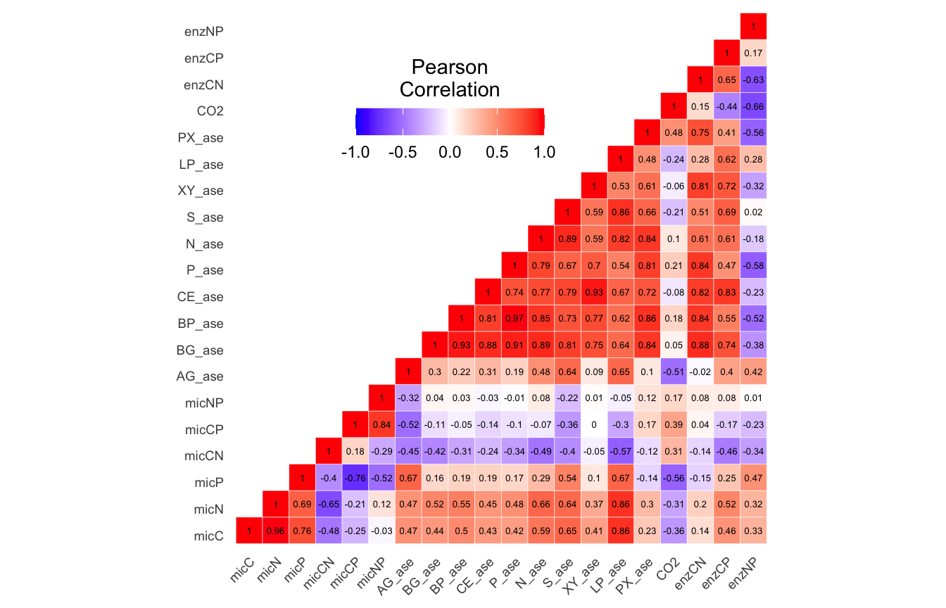
Autocorrelation Tests

Next, we test the metadata for autocorrelations. Do we do this on the original data or the transformed data? No idea, so let’s do both.

Split Metadata

We need to split the data into different groups.

Environmental and edaphic properties
Microbial functional responses
Temperature adaptation properties

We first create lists of metadata parameters.

Show the code

div <- c("PLOT", "TREAT", "TREAT_T", "PAIR", "Observed", "Shannon_exp", 
         "InvSimpson", "ATAP")

edaphic <- c("AST", "H2O", "N", "P", "Al", 
             "Ca", "Fe", "K", "Mg", "Mn", "Na", "TEB", "ECEC", "pH", 
             "NH4", "NO3", "PO4", "DOC", "DON", "DOCN")

soil_funct <- c("micC", "micN", "micP", "micCN", "micCP", "micNP", 
                "AG_ase", "BG_ase", "BP_ase", "CE_ase", "P_ase", "N_ase", 
                "S_ase", "XY_ase",  "LP_ase", "PX_ase", "CO2", 
                "enzCN", "enzCP", "enzNP")

temp_adapt <- c("AG_Q10", "BG_Q10", "BP_Q10", "CE_Q10", "P_Q10", "N_Q10", 
                "S_Q10", "XY_Q10", "LP_Q10", "PX_Q10", "CUEcn", "CUEcp", 
                "NUE","PUE", "Tmin", "SI")

md_groups <- c("edaphic", "soil_funct", "temp_adapt")

# NoT uSed: minPO4, minNH4, minNO3, minTIN

And then use the lists to split the data sets by metadata group. Here, we do this for the original metadata and the metadata after normalization.

Show the code

select_md <- c("ssu18_select_mc", "ssu18_select_mc_norm")
for (i in select_md) {
   #tmp_get <- get(purrr::map_chr(i, ~ paste0(i, "_mc")))
   tmp_get <- get(i)
   tmp_md_all <- tmp_get$map_loaded
   tmp_div <- tmp_md_all %>% dplyr::select(all_of(div))
   tmp_div <- tmp_div %>% tibble::rownames_to_column("SampleID")
## edaphic      
   tmp_sub_edaphic <- tmp_md_all %>% dplyr::select(all_of(edaphic))
   tmp_sub_edaphic <- tmp_sub_edaphic %>% tibble::rownames_to_column("SampleID")
   tmp_edaphic <- dplyr::left_join(tmp_div, tmp_sub_edaphic, by = "SampleID")
   tmp_edaphic <- tmp_edaphic %>% tibble::column_to_rownames("SampleID")
## soil_funct
   tmp_sub_soil_funct <- tmp_md_all %>% dplyr::select(all_of(soil_funct))
   tmp_sub_soil_funct <- tmp_sub_soil_funct %>% tibble::rownames_to_column("SampleID")
   tmp_soil_funct <- dplyr::left_join(tmp_div, tmp_sub_soil_funct, by = "SampleID")
   tmp_soil_funct <- tmp_soil_funct %>% tibble::column_to_rownames("SampleID")      
## temp_adapt
   tmp_sub_temp_adapt <- tmp_md_all %>% dplyr::select(all_of(temp_adapt))
   tmp_sub_temp_adapt <- tmp_sub_temp_adapt %>% tibble::rownames_to_column("SampleID")
   tmp_temp_adapt <- dplyr::left_join(tmp_div, tmp_sub_temp_adapt, by = "SampleID")
   tmp_temp_adapt <- tmp_temp_adapt %>% tibble::column_to_rownames("SampleID")      
## combine
   tmp_list <- list(data_loaded = ssu18_select_mc$data_loaded, 
                    map_loaded = ssu18_select_mc$map_loaded, 
                    taxonomy_loaded = ssu18_select_mc$taxonomy_loaded,
                    edaphic = tmp_edaphic, 
                    soil_funct = tmp_soil_funct, 
                    temp_adapt = tmp_temp_adapt)
   tmp_name <- purrr::map_chr(i, ~ paste0(., "_split"))
   print(tmp_name)
   assign(tmp_name, tmp_list)
   rm(list = ls(pattern = "tmp_"))
}

Generate Autocorrelation Plots

A little housekeeping to get rid of parameters we don’t need (e.g., plot number, pair, etc.).

Show the code

edaphic_cor <- ssu18_select_mc_split$edaphic
edaphic_cor[,1:8] <- NULL
edaphic_norm_cor <- ssu18_select_mc_norm_split$edaphic
edaphic_norm_cor[,1:8] <- NULL

soil_funct_cor <- ssu18_select_mc_split$soil_funct
soil_funct_cor[,1:8] <- NULL
soil_funct_norm_cor <- ssu18_select_mc_norm_split$soil_funct
soil_funct_norm_cor[,1:8] <- NULL

temp_adapt_cor <- ssu18_select_mc_split$temp_adapt
temp_adapt_cor[,1:8] <- NULL
temp_adapt_norm_cor <- ssu18_select_mc_norm_split$temp_adapt
temp_adapt_norm_cor[,1:8] <- NULL

And finally the code to create the plots.

Show the code

for (i in objects(pattern = "_cor$")) {
  tmp_get <- get(i)
  tmp_cormat <- round(cor(tmp_get), 2)
  tmp_melted_cormat <- reshape2::melt(tmp_cormat)
  
  tmp_get_lower_tri <- function(tmp_cormat){
    tmp_cormat[upper.tri(tmp_cormat)] <- NA
    return(tmp_cormat)
    }
  # Get upper triangle of the correlation matrix
  tmp_get_upper_tri <- function(tmp_cormat){
    tmp_cormat[lower.tri(tmp_cormat)] <- NA
    return(tmp_cormat)
    }
  tmp_upper_tri <- tmp_get_upper_tri(tmp_cormat)
  tmp_melted_cormat <- reshape2::melt(tmp_upper_tri, na.rm = TRUE)
  ggplot(data = tmp_melted_cormat, aes(x = Var1, y = Var2, fill = value)) + 
    geom_tile()
  
  tmp_ggheatmap <- ggplot(data = tmp_melted_cormat, aes(Var2, Var1, fill = value)) +
    geom_tile(color = "white") +
    scale_fill_gradient2(low = "blue", high = "red", mid = "white", 
                         midpoint = 0, limit = c(-1,1), space = "Lab", 
                         name="Pearson\nCorrelation") +
    theme_minimal() + 
    theme(axis.text.x = element_text(angle = 45, vjust = 1, 
                                     size = 7, hjust = 1),
          axis.text.y = element_text(vjust = 1, size = 7, hjust = 1)) + 
    coord_fixed() + 
    geom_text(aes(Var2, Var1, label = value), color = "black", size = 1.75) +
    theme(
      axis.title.x = element_blank(),
      axis.title.y = element_blank(),
      panel.grid.major = element_blank(),
      panel.border = element_blank(),
      panel.background = element_blank(),
      axis.ticks = element_blank(),
      legend.justification = c(1, 0),
      legend.position = c(0.6, 0.7),
      legend.direction = "horizontal") +
      guides(fill = guide_colorbar(barwidth = 7, barheight = 1,
                                   title.position = "top", 
                                   title.hjust = 0.5))
  tmp_name <- purrr::map_chr(i, ~ paste0(., "_ggheatmap"))
  assign(tmp_name, tmp_ggheatmap)
  print(tmp_name)
  rm(list = ls(pattern = "tmp_"))
}  
objects(pattern = "_ggheatmap")

(16S rRNA) Figure 1 | Results of autocorrelation analysis for non-normalized Environmental and edaphic parameters.

(16S rRNA) Figure 2 | Results of autocorrelation analysis for normalized Environmental and edaphic parameters.

Functional responses
Functional responses (normalized)

(16S rRNA) Figure 3 | Results of autocorrelation analysis for non-normalized Functional response parameters.

(16S rRNA) Figure 4 | Results of autocorrelation analysis for normalized Functional response parameters.

Temperature adaptation
Temperature adaptation (normalized)

(16S rRNA) Figure 5 | Results of autocorrelation analysis for non-normalized Temperature adaptation parameters.

(16S rRNA) Figure 6 | Results of autocorrelation analysis for normalized Temperature adaptation parameters.

Now we can remove parameters based on the autocorrelation analysis:

Environmental and edaphic properties: TEB, DON, Na, Al, Ca.
Microbial functional responses: micN, micNP, enzCN, enzCP, BP_ase, CE_ase, LP_ase, N_ase, P_ase.
Temperature adaptation properties: NUE, PUE, SI.

edaphic_remove <- c("TEB", "DON", "Na", "Al", "Ca")
soil_funct_remove <- c("micN", "micNP", "enzCN", "enzCP", "BP_ase", 
                       "CE_ase", "LP_ase", "N_ase", "P_ase")
temp_adapt_remove <- c("NUE", "PUE", "SI")

Show the code

tmp_df <- ssu18_select_mc_split
tmp_df$edaphic <- tmp_df$edaphic[, ! names(tmp_df$edaphic) %in%  edaphic_remove]
tmp_df$soil_funct <- tmp_df$soil_funct[, ! names(tmp_df$soil_funct) %in%  soil_funct_remove]
tmp_df$temp_adapt <- tmp_df$temp_adapt[, ! names(tmp_df$temp_adapt) %in%  temp_adapt_remove]
ssu18_select_mc_split_no_ac <- tmp_df
rm(list = ls(pattern = "tmp_"))

tmp_df <- ssu18_select_mc_norm_split
tmp_df$edaphic <- tmp_df$edaphic[, ! names(tmp_df$edaphic) %in%  edaphic_remove]
tmp_df$soil_funct <- tmp_df$soil_funct[, ! names(tmp_df$soil_funct) %in%  soil_funct_remove]
tmp_df$temp_adapt <- tmp_df$temp_adapt[, ! names(tmp_df$temp_adapt) %in%  temp_adapt_remove]
ssu18_select_mc_norm_split_no_ac <- tmp_df
rm(list = ls(pattern = "tmp_"))

Dissimilarity Correlation Tests

Let’s see if any on the metadata groups are significantly correlated with the community data. Basically, we create distance matrices for the community data and each metadata group and then run Mantel tests for all comparisons. For the community data we calculate Bray-Curtis distances for the community data and Euclidean distances for the metadata. We use the function mantel.test from the ape package and mantel from the vegan package for the analyses.

In summary, we test both mantel.test and mantel on Bray-Curtis distance community distances against Euclidean distances for each metadata group (edaphic, soil_funct, temp_adapt) a) before normalizing and before removing autocorrelated parameters, b) before normalizing and after removing autocorrelated parameters, c) after normalizing and before removing autocorrelated parameters, and d) after normalizing and after removing autocorrelated parameters.

Show the code

man_df <- c("ssu18_select_mc_split", "ssu18_select_mc_split_no_ac", 
            "ssu18_select_mc_norm_split", "ssu18_select_mc_norm_split_no_ac")

for (i in man_df) {
  tmp_get <- get(i)
  tmp_dm_otu <- as.matrix(vegdist(t(tmp_get$data_loaded), 
                             method = "bray", binary = FALSE, 
                             diag = TRUE, upper = TRUE, na.rm = FALSE))
# EDAPHIC
  tmp_dm_md_edaphic <- as.matrix(vegdist(tmp_get$edaphic[, 8:ncol(tmp_get$edaphic)], 
                                    method ="euclidean", binary = FALSE, 
                                    diag = TRUE, upper = TRUE, na.rm = FALSE))

  tmp_man1_edaphic <- mantel.test(tmp_dm_otu, tmp_dm_md_edaphic, nperm = 999, 
                             graph = FALSE, alternative = "two.sided")
  tmp_man2_edaphic <- mantel(tmp_dm_otu, tmp_dm_md_edaphic, permutations = 999)
# SOIL FUNCT
  tmp_dm_md_soil_funct <- as.matrix(vegdist(tmp_get$soil_funct[, 8:ncol(tmp_get$soil_funct)], 
                                       method = "euclidean", binary = FALSE, 
                                       diag = TRUE, upper = TRUE, na.rm = FALSE))

  tmp_man1_soil_funct <- mantel.test(tmp_dm_otu, tmp_dm_md_soil_funct, nperm = 999, 
                                graph = FALSE, alternative = "two.sided")
  tmp_man2_soil_funct <- mantel(tmp_dm_otu, tmp_dm_md_soil_funct, permutations = 999)

# TEMP ADAPT
  tmp_dm_md_temp_adapt <- as.matrix(vegdist(tmp_get$temp_adapt[, 8:ncol(tmp_get$temp_adapt)], 
                                       method = "euclidean", binary = FALSE, 
                                       diag = TRUE, upper = TRUE, na.rm = FALSE))

  tmp_man1_temp_adapt <- mantel.test(tmp_dm_otu, tmp_dm_md_temp_adapt, nperm = 999, 
                                graph = FALSE, alternative = "two.sided")
  tmp_man2_temp_adapt <- mantel(tmp_dm_otu, tmp_dm_md_temp_adapt, permutations = 999)

  tmp_name <- purrr::map_chr(i, ~ paste0(., "_mantel_tests"))
  tmp_df <- list(edaphic_ape_man = tmp_man1_edaphic, 
                 edaphic_vegan_man = tmp_man2_edaphic,
                 soil_funct_ape_man = tmp_man1_soil_funct, 
                 soil_funct_vegan_man = tmp_man2_soil_funct,
                 temp_adapt_ape_man = tmp_man1_temp_adapt, 
                 temp_adapt_vegan_man = tmp_man2_temp_adapt)
  assign(tmp_name, tmp_df)
  print(tmp_name)
  rm(list = ls(pattern = "tmp_"))
}

Dissimilarity Correlation Results

(16S rRNA) Table 4 | Summary of Dissimilarity Correlation Tests using mantel.test from the ape package and mantel from the vegan. P-values in red indicate significance (p-value < 0.05)

Moving on.

Best Subset of Variables

Now we want to know which of the metadata parameters are the most strongly correlated with the community data. For this we use the bioenv function from the vegan package. bioenv—Best Subset of Environmental Variables with Maximum (Rank) Correlation with Community Dissimilarities—finds the best subset of environmental variables, so that the Euclidean distances of scaled environmental variables have the maximum (rank) correlation with community dissimilarities.

Next we will use the metadata set where autocorrelated parameters were removed and the remainder of the parameters were normalized (where applicable based on the Shapiro tests).

We run bioenv against the three groups of metadata parameters. We then run bioenv again, but this time against the individual parameters identified as significantly correlated.

Edaphic Properties

Show the code

tmp_comm <- data.frame(t(ssu18_select_mc_norm_split_no_ac$data_loaded))
tmp_env <- data.frame(ssu18_select_mc_norm_split_no_ac$edaphic)
tmp_env[,1:8] <- NULL

edaphic_bioenv <- bioenv(wisconsin(tmp_comm), tmp_env, 
                         method = "spearman", index = "bray", 
                         upto = ncol(tmp_env), metric = "euclidean")

bioenv_list <- edaphic_bioenv$models[[edaphic_bioenv$whichbest]]$best
bioenv_best <- bioenvdist(edaphic_bioenv, which = "best")

for (i in bioenv_list) {
       tmp_dp <- data.frame(edaphic_bioenv$x)
       tmp_md <- as.matrix(vegdist(tmp_dp[[i]], 
                                   method = "euclidean", binary = FALSE, 
                                   diag = TRUE, upper = TRUE, na.rm = FALSE))
       tmp_man <- mantel(bioenv_best, tmp_md, 
                         permutations = 999, method = "spearman")
       tmp_md_name <- names(tmp_dp)[[i]]
       tmp_name <- purrr::map_chr(tmp_md_name, ~ paste0(., "_bioenv_mantel_test"))
       assign(tmp_name, tmp_man)
       rm(list = ls(pattern = "tmp_"))
}
objects(pattern = "_bioenv_mantel_test")
edaphic_bioenv_ind_mantel <- list(AST = AST_bioenv_mantel_test)
rm(list = ls(pattern = "_bioenv_mantel_test"))


Call:
bioenv(comm = wisconsin(tmp_comm), env = tmp_env, method = "spearman",      index = "bray", upto = ncol(tmp_env), metric = "euclidean") 

Subset of environmental variables with best correlation to community data.

Correlations:    spearman 
Dissimilarities: bray 
Metric:          euclidean 

Best model has 1 parameters (max. 15 allowed):
AST
with correlation  0.6808861

Show the results of individual edaphic metadata Mantel tests

$AST

Mantel statistic based on Spearman's rank correlation rho 

Call:
mantel(xdis = bioenv_best, ydis = tmp_md, method = "spearman",      permutations = 999) 

Mantel statistic r:     1 
      Significance: 0.001 

Upper quantiles of permutations (null model):
  90%   95% 97.5%   99% 
0.177 0.226 0.271 0.326 
Permutation: free
Number of permutations: 999

bioenv found the following edaphic properties significantly correlated with the community data: AST

Soil Functional Response

Show the code

tmp_comm <- data.frame(t(ssu18_select_mc_norm_split_no_ac$data_loaded))
tmp_env <- data.frame(ssu18_select_mc_norm_split_no_ac$soil_funct)
tmp_env[,1:8] <- NULL

soil_funct_bioenv <- bioenv(wisconsin(tmp_comm), tmp_env, 
                         method = "spearman", index = "bray", 
                         upto = ncol(tmp_env), metric = "euclidean")

bioenv_list <- soil_funct_bioenv$models[[soil_funct_bioenv$whichbest]]$best
bioenv_best <- bioenvdist(soil_funct_bioenv, which = "best")

for (i in bioenv_list) {
       tmp_dp <- data.frame(soil_funct_bioenv$x)
       tmp_md <- as.matrix(vegdist(tmp_dp[[i]], 
                                   method = "euclidean", binary = FALSE, 
                                   diag = TRUE, upper = TRUE, na.rm = FALSE))
       tmp_man <- mantel(bioenv_best, tmp_md, 
                         permutations = 999, method = "spearman")
       tmp_md_name <- names(tmp_dp)[[i]]
       tmp_name <- purrr::map_chr(tmp_md_name, ~ paste0(., "_bioenv_mantel_test"))
       assign(tmp_name, tmp_man)
       rm(list = ls(pattern = "tmp_"))
}
objects(pattern = "_bioenv_mantel_test")

soil_funct_bioenv_ind_mantel <- list(AG_ase = AG_ase_bioenv_mantel_test, 
                                     enzNP = enzNP_bioenv_mantel_test, 
                                     S_ase = S_ase_bioenv_mantel_test, 
                                     PX_ase = PX_ase_bioenv_mantel_test,
                                     XY_ase = XY_ase_bioenv_mantel_test)
rm(list = ls(pattern = "_bioenv_mantel_test"))


Call:
bioenv(comm = wisconsin(tmp_comm), env = tmp_env, method = "spearman",      index = "bray", upto = ncol(tmp_env), metric = "euclidean") 

Subset of environmental variables with best correlation to community data.

Correlations:    spearman 
Dissimilarities: bray 
Metric:          euclidean 

Best model has 5 parameters (max. 11 allowed):
AG_ase S_ase XY_ase PX_ase enzNP
with correlation  0.7727866

Show the results of individual functional response metadata Mantel tests

$AG_ase

Mantel statistic based on Spearman's rank correlation rho 

Call:
mantel(xdis = bioenv_best, ydis = tmp_md, method = "spearman",      permutations = 999) 

Mantel statistic r: 0.5588 
      Significance: 0.001 

Upper quantiles of permutations (null model):
  90%   95% 97.5%   99% 
0.186 0.235 0.281 0.330 
Permutation: free
Number of permutations: 999


$enzNP

Mantel statistic based on Spearman's rank correlation rho 

Call:
mantel(xdis = bioenv_best, ydis = tmp_md, method = "spearman",      permutations = 999) 

Mantel statistic r: 0.4623 
      Significance: 0.006 

Upper quantiles of permutations (null model):
  90%   95% 97.5%   99% 
0.219 0.280 0.336 0.413 
Permutation: free
Number of permutations: 999


$S_ase

Mantel statistic based on Spearman's rank correlation rho 

Call:
mantel(xdis = bioenv_best, ydis = tmp_md, method = "spearman",      permutations = 999) 

Mantel statistic r: 0.6139 
      Significance: 0.001 

Upper quantiles of permutations (null model):
  90%   95% 97.5%   99% 
0.223 0.305 0.384 0.466 
Permutation: free
Number of permutations: 999


$PX_ase

Mantel statistic based on Spearman's rank correlation rho 

Call:
mantel(xdis = bioenv_best, ydis = tmp_md, method = "spearman",      permutations = 999) 

Mantel statistic r: 0.6115 
      Significance: 0.001 

Upper quantiles of permutations (null model):
  90%   95% 97.5%   99% 
0.176 0.222 0.289 0.346 
Permutation: free
Number of permutations: 999


$XY_ase

Mantel statistic based on Spearman's rank correlation rho 

Call:
mantel(xdis = bioenv_best, ydis = tmp_md, method = "spearman",      permutations = 999) 

Mantel statistic r: 0.456 
      Significance: 0.002 

Upper quantiles of permutations (null model):
  90%   95% 97.5%   99% 
0.189 0.258 0.304 0.347 
Permutation: free
Number of permutations: 999

bioenv found the following soil functions significantly correlated with the community data: AG_ase, enzNP, S_ase, PX_ase, XY_ase

Temperature Adaptation

Show the code

tmp_comm <- data.frame(t(ssu18_select_mc_norm_split_no_ac$data_loaded))
tmp_env <- data.frame(ssu18_select_mc_norm_split_no_ac$temp_adapt)
tmp_env[,1:8] <- NULL

temp_adapt_bioenv <- bioenv(wisconsin(tmp_comm), tmp_env, 
                         method = "spearman", index = "bray", 
                         upto = ncol(tmp_env), metric = "euclidean")

bioenv_list <- temp_adapt_bioenv$models[[temp_adapt_bioenv$whichbest]]$best
bioenv_best <- bioenvdist(temp_adapt_bioenv, which = "best")

for (i in bioenv_list) {
       tmp_dp <- data.frame(temp_adapt_bioenv$x)
       tmp_md <- as.matrix(vegdist(tmp_dp[[i]], 
                                   method = "euclidean", binary = FALSE, 
                                   diag = TRUE, upper = TRUE, na.rm = FALSE))
       tmp_man <- mantel(bioenv_best, tmp_md, 
                         permutations = 999, method = "spearman")
       tmp_md_name <- names(tmp_dp)[[i]]
       tmp_name <- purrr::map_chr(tmp_md_name, ~ paste0(., "_bioenv_mantel_test"))
       assign(tmp_name, tmp_man)
       rm(list = ls(pattern = "tmp_"))
}
objects(pattern = "_bioenv_mantel_test")

temp_adapt_bioenv_ind_mantel <- list(CUEcp = CUEcp_bioenv_mantel_test, 
                                     LP_Q10 = LP_Q10_bioenv_mantel_test, 
                                     P_Q10 = P_Q10_bioenv_mantel_test, 
                                     S_Q10 = S_Q10_bioenv_mantel_test, 
                                     Tmin = Tmin_bioenv_mantel_test)
rm(list = ls(pattern = "_bioenv_mantel_test"))


Call:
bioenv(comm = wisconsin(tmp_comm), env = tmp_env, method = "spearman",      index = "bray", upto = ncol(tmp_env), metric = "euclidean") 

Subset of environmental variables with best correlation to community data.

Correlations:    spearman 
Dissimilarities: bray 
Metric:          euclidean 

Best model has 5 parameters (max. 13 allowed):
P_Q10 S_Q10 LP_Q10 CUEcp Tmin
with correlation  0.4237093

Show the results of individual temperature adaptation metadata Mantel tests

$CUEcp

Mantel statistic based on Spearman's rank correlation rho 

Call:
mantel(xdis = bioenv_best, ydis = tmp_md, method = "spearman",      permutations = 999) 

Mantel statistic r: 0.325 
      Significance: 0.013 

Upper quantiles of permutations (null model):
  90%   95% 97.5%   99% 
0.188 0.226 0.280 0.331 
Permutation: free
Number of permutations: 999


$LP_Q10

Mantel statistic based on Spearman's rank correlation rho 

Call:
mantel(xdis = bioenv_best, ydis = tmp_md, method = "spearman",      permutations = 999) 

Mantel statistic r: 0.3772 
      Significance: 0.005 

Upper quantiles of permutations (null model):
  90%   95% 97.5%   99% 
0.203 0.272 0.306 0.351 
Permutation: free
Number of permutations: 999


$P_Q10

Mantel statistic based on Spearman's rank correlation rho 

Call:
mantel(xdis = bioenv_best, ydis = tmp_md, method = "spearman",      permutations = 999) 

Mantel statistic r: 0.5177 
      Significance: 0.001 

Upper quantiles of permutations (null model):
  90%   95% 97.5%   99% 
0.158 0.211 0.261 0.309 
Permutation: free
Number of permutations: 999


$S_Q10

Mantel statistic based on Spearman's rank correlation rho 

Call:
mantel(xdis = bioenv_best, ydis = tmp_md, method = "spearman",      permutations = 999) 

Mantel statistic r: 0.4395 
      Significance: 0.001 

Upper quantiles of permutations (null model):
  90%   95% 97.5%   99% 
0.159 0.205 0.252 0.301 
Permutation: free
Number of permutations: 999


$Tmin

Mantel statistic based on Spearman's rank correlation rho 

Call:
mantel(xdis = bioenv_best, ydis = tmp_md, method = "spearman",      permutations = 999) 

Mantel statistic r: 0.4044 
      Significance: 0.005 

Upper quantiles of permutations (null model):
  90%   95% 97.5%   99% 
0.207 0.267 0.305 0.359 
Permutation: free
Number of permutations: 999

bioenv found the following temperature adaptations significantly correlated with the community data: CUEcp, LP_Q10, P_Q10, S_Q10, Tmin

Distance-based Redundancy

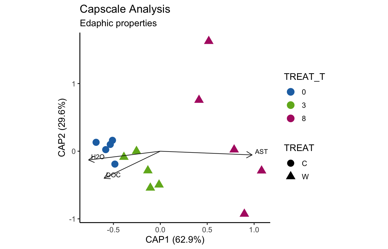
Now we turn our attention to distance-based redundancy analysis (dbRDA), an ordination method similar to Redundancy Analysis (rda) but it allows non-Euclidean dissimilarity indices, such as Manhattan or Bray–Curtis distance. For this, we use capscale from the vegan package. capscale is a constrained versions of metric scaling (principal coordinates analysis), which are based on the Euclidean distance but can be used, and are more useful, with other dissimilarity measures. The functions can also perform unconstrained principal coordinates analysis, optionally using extended dissimilarities.

For each of the three metadata subsets, we perform the following steps:

Run rankindex to compare metadata and community dissimilarity indices for gradient detection. This will help us select the best dissimilarity metric to use.
Run capscale for distance-based redundancy analysis.
Run envfit to fit environmental parameters onto the ordination. This function basically calculates correlation scores between the metadata parameters and the ordination axes.
Select metadata parameters significant for bioenv (see above) and/or envfit analyses.
Run envfit on ASVs.
Plot the ordination and vector overlays.

Edaphic Properties

Show the code

tmp_md <- ssu18_select_mc_norm_split_no_ac$edaphic
tmp_md$TREAT_T <- as.character(tmp_md$TREAT_T)
tmp_comm <- data.frame(t(ssu18_select_mc_norm_split_no_ac$data_loaded))
edaphic_rank <- rankindex(tmp_md[, 8:ncol(tmp_md)], tmp_comm, 
          indices = c("euc", "man", "gow","bra", "kul"), 
          stepacross = FALSE, method = "spearman")

      euc       man       gow       bra       kul 
0.3171263 0.4336927 0.1028302 0.4336927 0.4336927

Let’s run capscale using Bray-Curtis. Note, we have 15 metadata parameters in this group but, for some reason, capscale only works with 13 parameters. This may have to do with degrees of freedom?

Starting properties: AST, H2O, N, P, Al, Ca, Fe, K, Mg, Mn, Na, TEB, ECEC, pH, NH4, NO3, PO4, DOC, DON, DOCN
Autocorrelated removed: TEB, DON, Na, Al, Ca
Remove for capscale: Mg, Mn

edaphic_cap <- capscale(tmp_comm ~ AST + H2O + N + P + Fe + K + ECEC + 
                                   pH + NH4 + NO3 + PO4 + DOC + DOCN, 
                        tmp_md, dist = "bray")
colnames(tmp_md)


Call: capscale(formula = tmp_comm ~ AST + H2O + N + P + Fe + K + ECEC + pH
+ NH4 + NO3 + PO4 + DOC + DOCN, data = tmp_md, distance = "bray")

              Inertia Proportion Rank
Total         1.67890    1.00000     
Constrained   1.63037    0.97110   13
Unconstrained 0.04853    0.02890    1

Inertia is squared Bray distance

-- NOTE:
Species scores projected from 'tmp_comm'

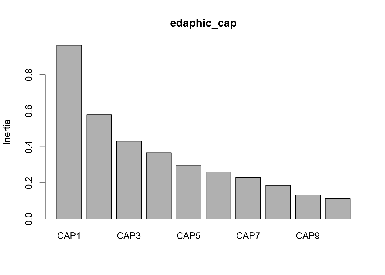
Eigenvalues for constrained axes:
  CAP1   CAP2   CAP3   CAP4   CAP5   CAP6   CAP7   CAP8   CAP9  CAP10  CAP11 
0.6287 0.2955 0.1984 0.1104 0.1085 0.0661 0.0536 0.0511 0.0359 0.0277 0.0247 
 CAP12  CAP13 
0.0218 0.0080 

Eigenvalues for unconstrained axes:
   MDS1 
0.04853

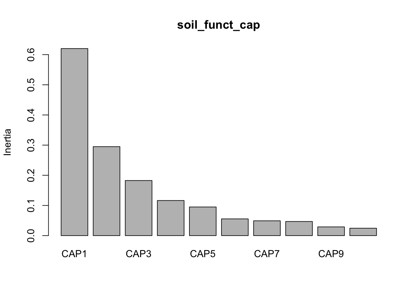
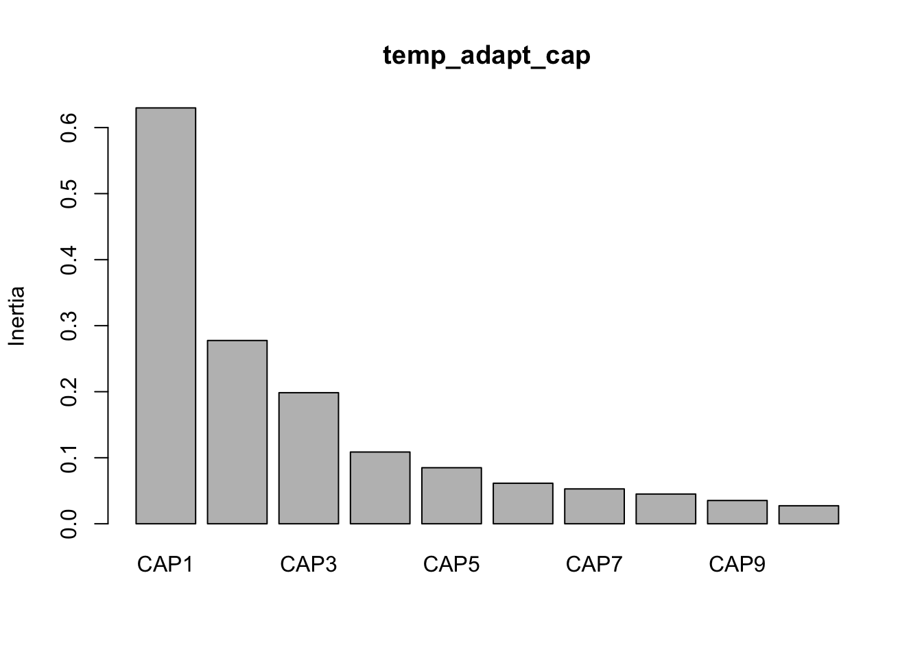
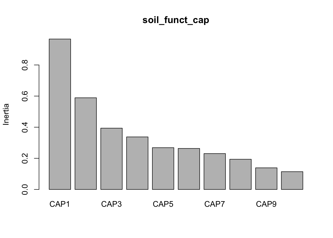
Now we can look at the variance against each principal component.

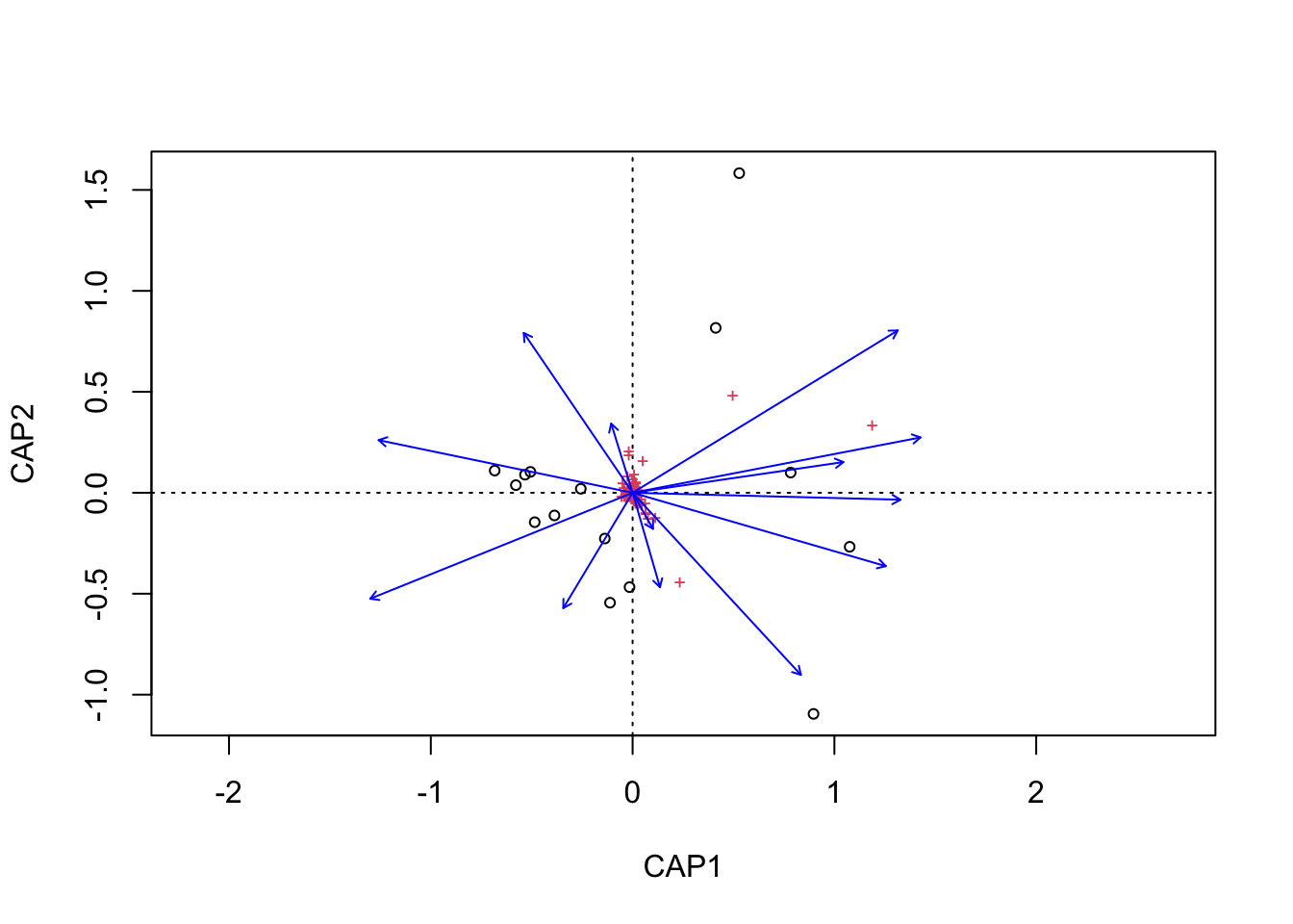
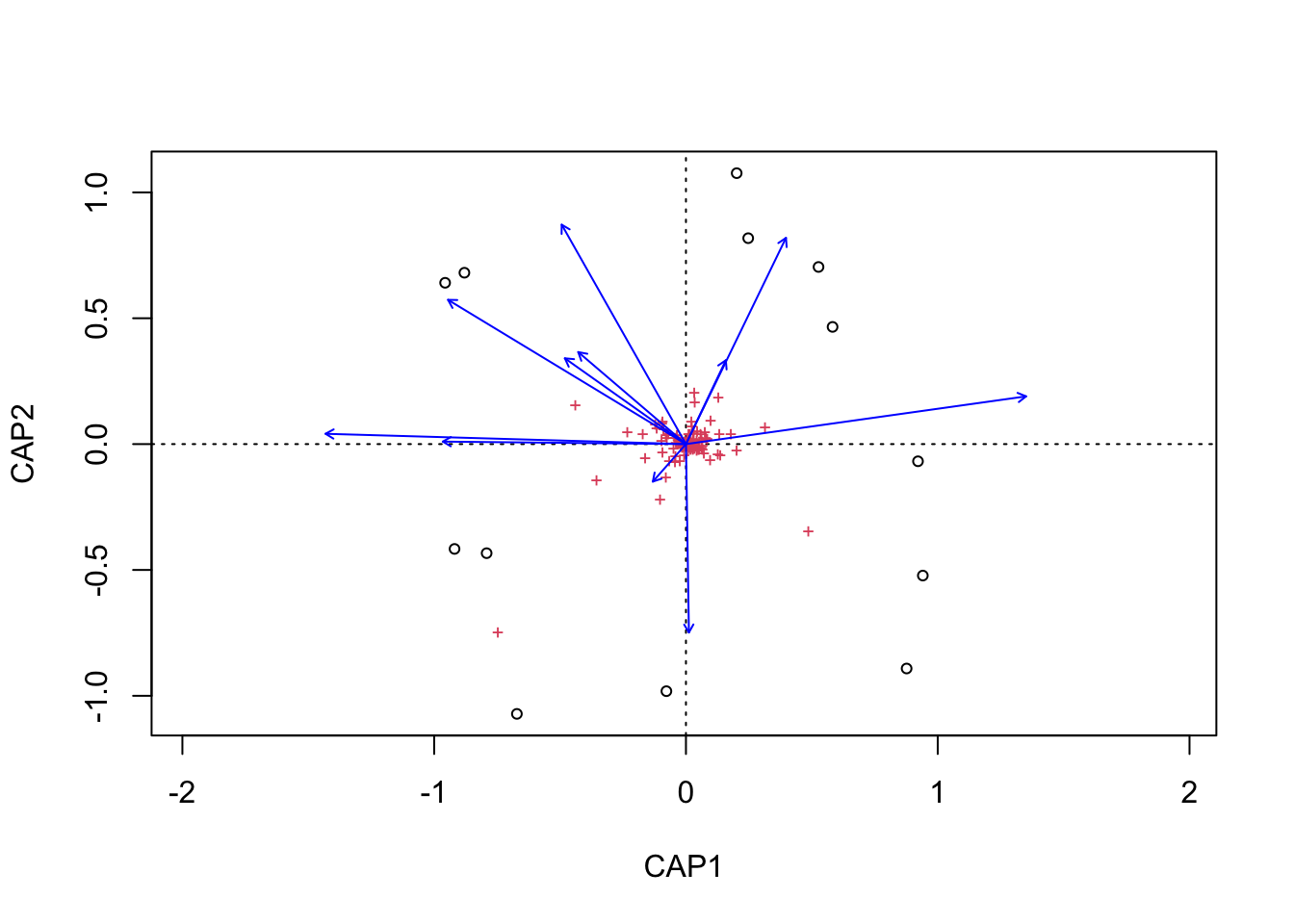
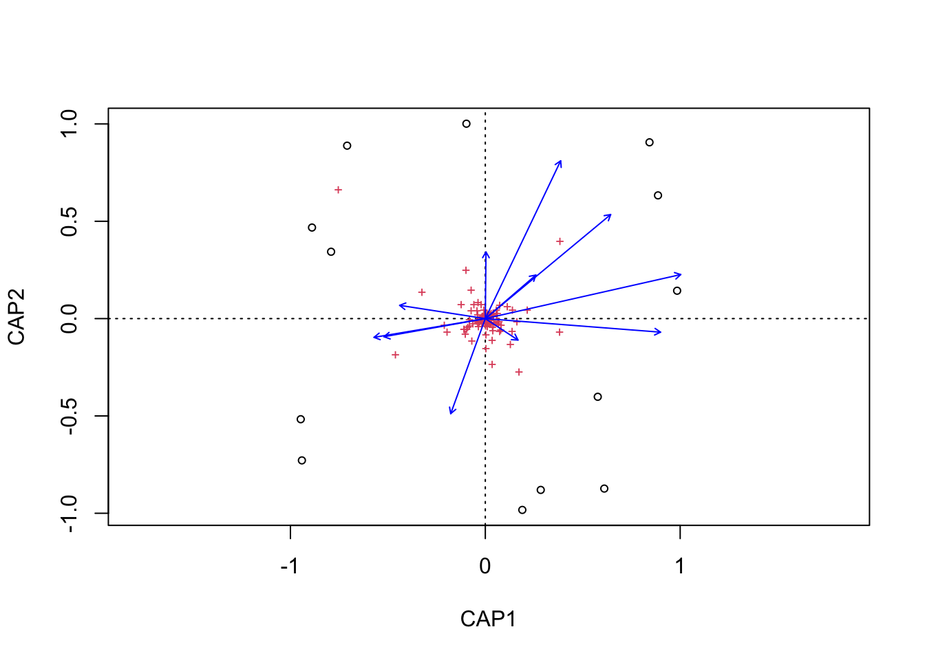
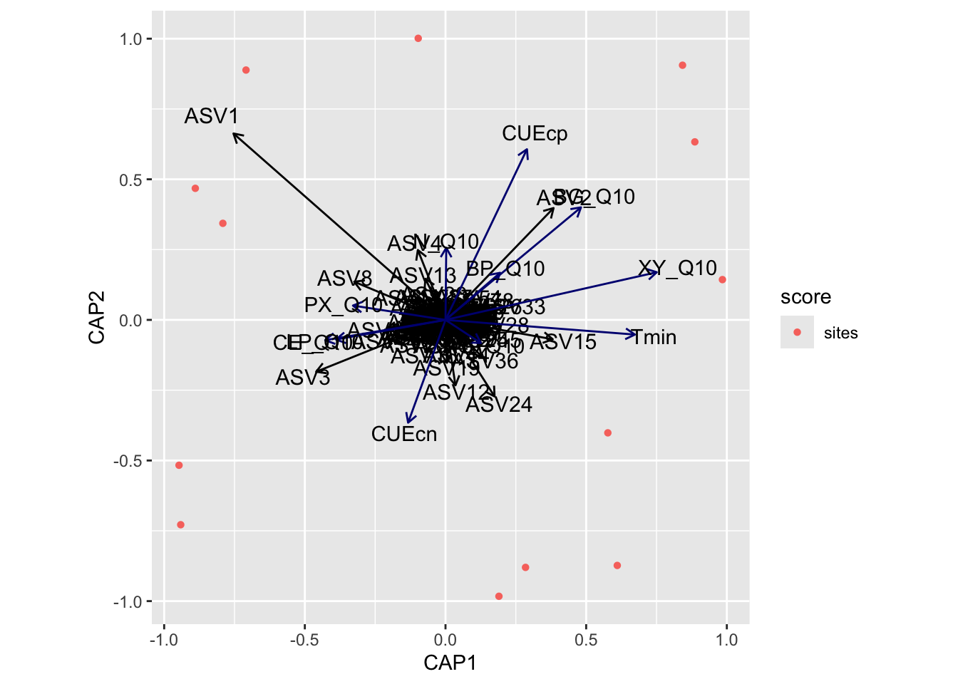
And then make some quick and dirty plots. This will also come in handy later when we need to parse out data a better plot visualization. The ggplot function autoplot stores these data in a more accessible way than the raw results from capscale

library(ggvegan)
base::plot(edaphic_cap)

tmp_auto_plt <- ggplot2::autoplot(edaphic_cap, arrows = TRUE)
tmp_auto_plt

Next, we need to grab capscale scores for the samples and create a data frame of the first two dimensions. We will also need to add some of the sample details to the data frame. For this we use the vegan function scores which gets species or site scores from the ordination.

Show the code

tmp_samp_scores <- dplyr::filter(tmp_auto_plt$plot_env$obj, Score == "sites")
tmp_samp_scores[,1] <- NULL
tmp_samp_scores <- tmp_samp_scores %>% dplyr::rename(SampleID = Label)

tmp_md_sub <- tmp_md[, 1:4]
tmp_md_sub <- tmp_md_sub %>% tibble::rownames_to_column("SampleID")
edaphic_plot_data <- dplyr::left_join(tmp_md_sub, tmp_samp_scores, by = "SampleID")

Now we have a new data frame that contains sample details and capscale values.

          SampleID PLOT TREAT TREAT_T PAIR        CAP1           CAP2
1  P10_D00_010_C0E  P10     C       0    E -0.51023381  0.16071056348
2  P02_D00_010_C0A  P02     C       0    A -0.48448722 -0.19055366181
3  P04_D00_010_C0B  P04     C       0    B -0.58218619  0.02325887477
4  P06_D00_010_C0C  P06     C       0    C -0.53370906  0.09973976767
5  P08_D00_010_C0D  P08     C       0    D -0.68492943  0.13143857676
6  P01_D00_010_W3A  P01     W       3    A -0.13286443 -0.28661650806
7  P03_D00_010_W3B  P03     W       3    B -0.25415783  0.00002258673
8  P05_D00_010_W3C  P05     W       3    C -0.38829574 -0.08695154559
9  P07_D00_010_W3D  P07     W       3    D -0.01360582 -0.49632449304
10 P09_D00_010_W3E  P09     W       3    E -0.10639798 -0.54219706978
11 P01_D00_010_W8A  P01     W       8    A  0.78689725  0.02214444812
12 P03_D00_010_W8B  P03     W       8    B  0.89574754 -0.92786190328
13 P05_D00_010_W8C  P05     W       8    C  1.07945322 -0.28874425650
14 P07_D00_010_W8D  P07     W       8    D  0.41234456  0.75597843926
15 P09_D00_010_W8E  P09     W       8    E  0.51642495  1.62595618128

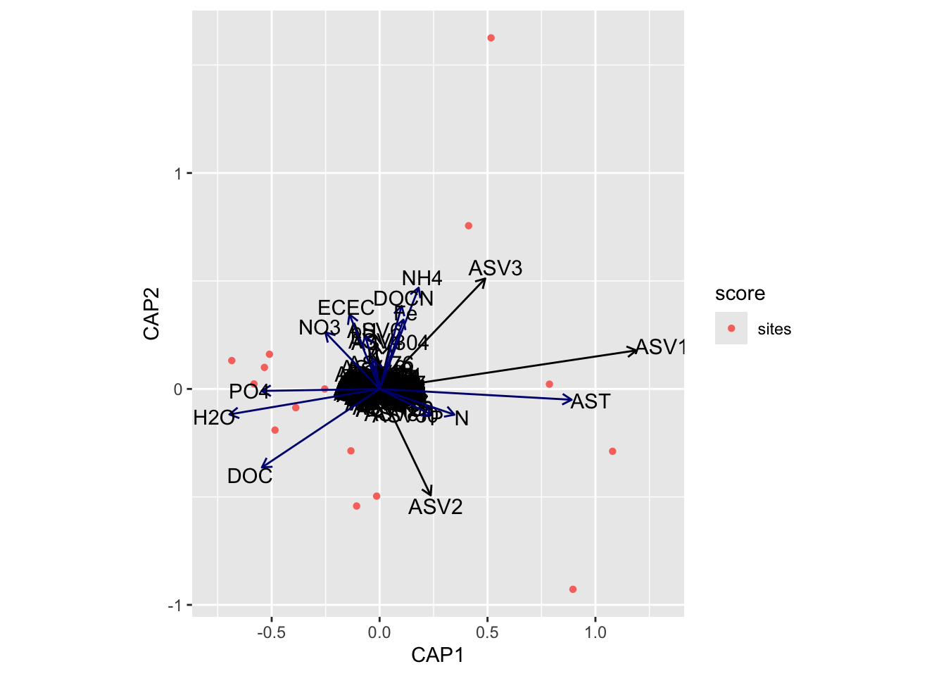
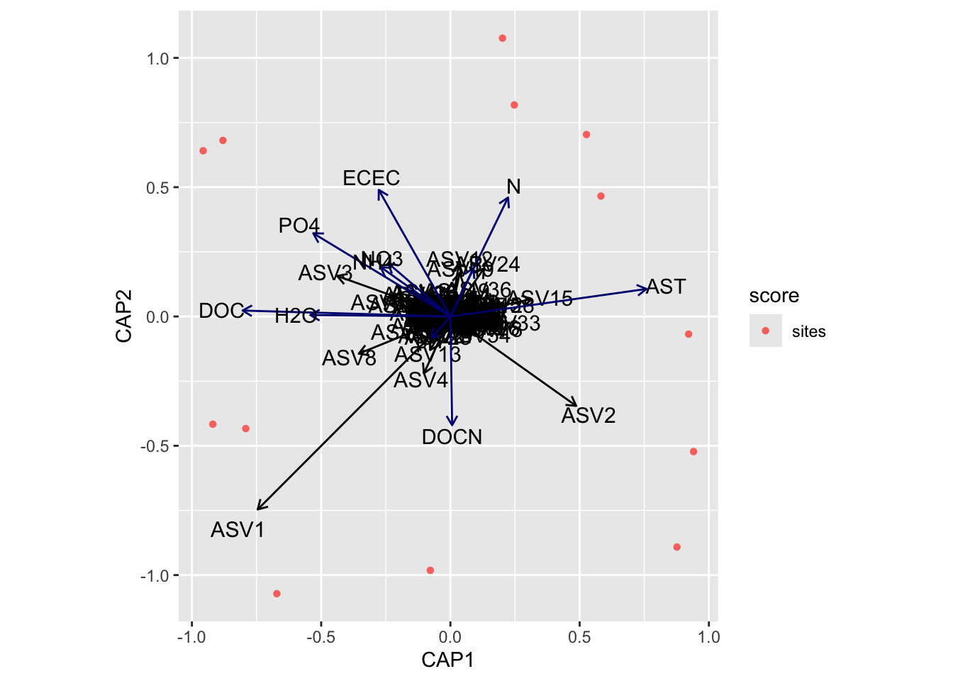
We can then do the same with the metadata vectors. Here though we only need the scores and parameter name.

Show the code

edaphic_md_scores <- dplyr::filter(tmp_auto_plt$plot_env$obj, Score == "biplot")
edaphic_md_scores[,1] <- NULL
edaphic_md_scores <- edaphic_md_scores %>% 
  dplyr::mutate(parameters = Label, .before = CAP1) %>%
  tibble::column_to_rownames("Label")

     parameters        CAP1         CAP2
AST         AST  0.97882379 -0.055074169
H2O         H2O -0.76548607 -0.129779379
N             N  0.38130076 -0.131035479
P             P  0.26536024 -0.132125558
Fe           Fe  0.12138586  0.353093177
K             K -0.02490580  0.151975508
ECEC       ECEC -0.15365335  0.379848234
pH           pH -0.07327989  0.272676813
NH4         NH4  0.19922925  0.516074241
NO3         NO3 -0.27681227  0.288729283
PO4         PO4 -0.60140669 -0.009980058
DOC         DOC -0.59979130 -0.399930429
DOCN       DOCN  0.11210058  0.422975484

Let’s run some quick correlations of metadata with ordination axes to see which parameters are significant. For this we use the vegan function envfit.

Show the code

tmp_samp_scores_sub <- edaphic_plot_data[, 6:7]
tmp_samp_scores_sub <- as.matrix(tmp_samp_scores_sub)
tmp_param_list <- edaphic_md_scores$parameters

tmp_md_sub <- subset(tmp_md,  select =  tmp_param_list)

envfit_edaphic_md <- envfit(tmp_samp_scores_sub, tmp_md_sub,
                 perm = 1000, choices = c(1, 2))


***VECTORS

         CAP1     CAP2     r2   Pr(>r)    
AST   0.99825 -0.05912 0.8287 0.000999 ***
H2O  -0.98657 -0.16333 0.5189 0.009990 ** 
N     0.94537 -0.32599 0.1403 0.398601    
P     0.89518 -0.44571 0.0759 0.602398    
Fe    0.32411  0.94602 0.1194 0.432567    
K    -0.16554  0.98620 0.0204 0.890110    
ECEC -0.37874  0.92550 0.1444 0.368631    
pH   -0.26344  0.96468 0.0685 0.672328    
NH4   0.35944  0.93317 0.2621 0.152847    
NO3  -0.69392  0.72006 0.1380 0.417582    
PO4  -0.99991 -0.01327 0.3118 0.090909 .  
DOC  -0.83396 -0.55183 0.4459 0.023976 *  
DOCN  0.25463  0.96704 0.1640 0.318681    
---
Signif. codes:  0 '***' 0.001 '**' 0.01 '*' 0.05 '.' 0.1 ' ' 1
Permutation: free
Number of permutations: 1000

Show the code

edaphic_md_signif_hits <- base::subset(envfit_edaphic_md$vectors$pvals, 
                                  c(envfit_edaphic_md$vectors$pvals 
                                  < 0.05 & envfit_edaphic_md$vectors$r > 0.4))
edaphic_md_signif_hits <- data.frame(edaphic_md_signif_hits)
edaphic_md_signif_hits <- rownames(edaphic_md_signif_hits)
edaphic_md_signif <- edaphic_md_scores[edaphic_md_scores$parameters %in% edaphic_md_signif_hits,]
edaphic_md_signif$parameters

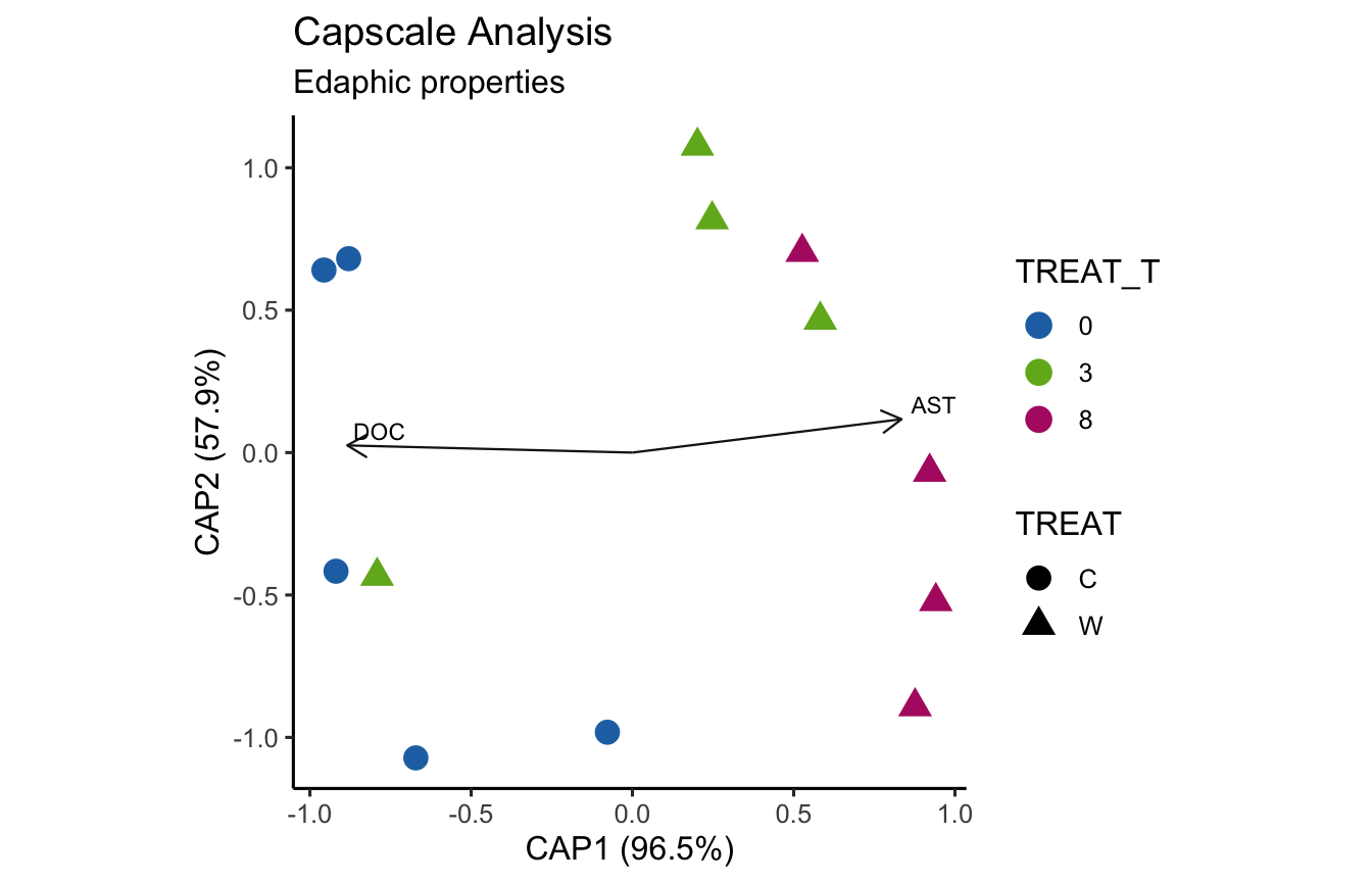
envfit found that AST, H2O, DOC were significantly correlated.

Now let’s see if the same parameters are significant for the envfit and bioenv analyses.

[1] "Significant parameters from bioenv analysis."
[1] "AST"
_____________________________________
[1] "Significant parameters from envfit analysis."
[1] "AST" "H2O" "DOC"
_____________________________________
[1] "Found in bioenv but not envfit."
character(0)
_____________________________________
[1] "Found in envfit but not bioenv."
[1] "H2O" "DOC"
_____________________________________
[1] "Found in envfit and bioenv."
[1] "AST" "H2O" "DOC"

Show the code

new_edaphic_md_signif_hits <- edaphic_sig_diff
#new_edaphic_md_signif_hits <- append(edaphic_md_signif_hits, edaphic_sig_diff)
edaphic_md_signif_all <- edaphic_md_scores[edaphic_md_scores$parameters %in% new_edaphic_md_signif_hits,]

Check. Next, we run envfit for the ASVs.

Show the code

envfit_edaphic_asv <- envfit(tmp_samp_scores_sub, 
                             tmp_comm[, order(colSums(-tmp_comm))][, 1:10],
                             perm = 1000, choices = c(1, 2))
edaphic_asv_scores <- dplyr::filter(tmp_auto_plt$plot_env$obj, Score == "species")
edaphic_asv_scores <- edaphic_asv_scores %>% 
  dplyr::mutate(parameters = Label, .before = CAP1) %>%
  tibble::column_to_rownames("Label")
edaphic_asv_scores[,1] <- NULL


***VECTORS

          CAP1     CAP2     r2   Pr(>r)    
ASV1   0.99502  0.09969 0.6491 0.005994 ** 
ASV2   0.54850 -0.83615 0.8984 0.000999 ***
ASV3   0.79245  0.60994 0.9429 0.000999 ***
ASV4  -0.12958  0.99157 0.2913 0.120879    
ASV5  -0.56363 -0.82603 0.1586 0.362637    
ASV6  -0.10651  0.99431 0.7559 0.000999 ***
ASV8  -0.84329  0.53746 0.4370 0.030969 *  
ASV7  -0.52510 -0.85104 0.0681 0.655345    
ASV9   0.51828 -0.85521 0.2559 0.185814    
ASV10 -0.34456  0.93876 0.8331 0.000999 ***
---
Signif. codes:  0 '***' 0.001 '**' 0.01 '*' 0.05 '.' 0.1 ' ' 1
Permutation: free
Number of permutations: 1000

Show the code

edaphic_asv_signif_hits <- base::subset(envfit_edaphic_asv$vectors$pvals, 
                                  c(envfit_edaphic_asv$vectors$pvals 
                                  < 0.05 & envfit_edaphic_asv$vectors$r > 0.5))
edaphic_asv_signif_hits <- data.frame(edaphic_asv_signif_hits)
edaphic_asv_signif_hits <- rownames(edaphic_asv_signif_hits)
edaphic_asv_signif <- edaphic_asv_scores[edaphic_asv_scores$parameters %in% edaphic_asv_signif_hits,]

      parameters        CAP1        CAP2 variable_type
ASV3        ASV3  0.48974117  0.51152737           ASV
ASV6        ASV6 -0.02123424  0.24919713           ASV
ASV2        ASV2  0.23670463 -0.49287683           ASV
ASV10      ASV10 -0.02578511  0.09240257           ASV
ASV1        ASV1  1.18949655  0.17867402           ASV

Show the code

edaphic_md_signif_all$variable_type <- "metadata"
edaphic_asv_signif$variable_type <- "ASV"
edaphic_bioplot_data <- rbind(edaphic_md_signif_all, edaphic_asv_signif)

The last thing to do is categorize parameters scores and ASV scores into different variable types for plotting.

Show the code

edaphic_bioplot_data_md <- subset(edaphic_bioplot_data, 
                                  edaphic_bioplot_data$variable_type == "metadata")
edaphic_bioplot_data_asv <- subset(edaphic_bioplot_data, 
                                   edaphic_bioplot_data$variable_type == "ASV")

Show the code for the plot

Soil Functional Response

Show the code

tmp_md <- ssu18_select_mc_norm_split_no_ac$soil_funct
tmp_md$TREAT_T <- as.character(tmp_md$TREAT_T)
tmp_comm <- data.frame(t(ssu18_select_mc_norm_split_no_ac$data_loaded))
soil_funct_rank <- rankindex(tmp_md[, 8:ncol(tmp_md)], tmp_comm, 
          indices = c("euc", "man", "gow","bra", "kul"), 
          stepacross = FALSE, method = "spearman")

      euc       man       gow       bra       kul 
0.5840452 0.7341800 0.2168775 0.7341800 0.7341800

Let’s run capscale using Bray-Curtis. Note, we have 11 metadata parameters in this group but, for some reason, capscale only works with 13 parameters. This may have to do with degrees of freedom?

Starting properties: micC, micN, micP, micCN, micCP, micNP, AG_ase, BG_ase, BP_ase, CE_ase, P_ase, N_ase, S_ase, XY_ase, LP_ase, PX_ase, CO2, enzCN, enzCP, enzNP
Autocorrelated removed: micN, micNP, enzCN, enzCP, BP_ase, CE_ase, LP_ase, N_ase, P_ase
Remove for capscale: NONE

soil_funct_cap <- capscale(tmp_comm ~ micC + micP + micCN + micCP + AG_ase + BG_ase + 
                                      S_ase + XY_ase + PX_ase + CO2 + enzNP, 
                           tmp_md, dist = "bray")


Call: capscale(formula = tmp_comm ~ micC + micP + micCN + micCP + AG_ase +
BG_ase + S_ase + XY_ase + PX_ase + CO2 + enzNP, data = tmp_md, distance =
"bray")

              Inertia Proportion Rank
Total         1.67890    1.00000     
Constrained   1.52672    0.90936   11
Unconstrained 0.15218    0.09064    3

Inertia is squared Bray distance

-- NOTE:
Species scores projected from 'tmp_comm'

Eigenvalues for constrained axes:
  CAP1   CAP2   CAP3   CAP4   CAP5   CAP6   CAP7   CAP8   CAP9  CAP10  CAP11 
0.6202 0.2950 0.1827 0.1164 0.0950 0.0555 0.0491 0.0468 0.0290 0.0246 0.0126 

Eigenvalues for unconstrained axes:
   MDS1    MDS2    MDS3 
0.06264 0.05568 0.03386

Now we can look at the variance against each principal component.

base::plot(soil_funct_cap)

tmp_auto_plt <- autoplot(soil_funct_cap, arrows = TRUE)
tmp_auto_plt

Show the code

tmp_samp_scores <- dplyr::filter(tmp_auto_plt$plot_env$obj, Score == "sites")
tmp_samp_scores[,1] <- NULL
tmp_samp_scores <- tmp_samp_scores %>% dplyr::rename(SampleID = Label)

tmp_md_sub <- tmp_md[, 1:4]
tmp_md_sub <- tmp_md_sub %>% tibble::rownames_to_column("SampleID")
soil_funct_plot_data <- dplyr::left_join(tmp_md_sub, tmp_samp_scores, 
                                         by = "SampleID")

Now we have a new data frame that contains sample details and capscale values.

          SampleID PLOT TREAT TREAT_T PAIR        CAP1        CAP2
1  P10_D00_010_C0E  P10     C       0    E -0.53163678  0.19467717
2  P02_D00_010_C0A  P02     C       0    A -0.49565928 -0.17246578
3  P04_D00_010_C0B  P04     C       0    B -0.58149488  0.04815608
4  P06_D00_010_C0C  P06     C       0    C -0.53700662  0.10581563
5  P08_D00_010_C0D  P08     C       0    D -0.69408551  0.15871504
6  P01_D00_010_W3A  P01     W       3    A -0.13789308 -0.32241637
7  P03_D00_010_W3B  P03     W       3    B -0.23991258 -0.02936566
8  P05_D00_010_W3C  P05     W       3    C -0.37861217 -0.07503400
9  P07_D00_010_W3D  P07     W       3    D -0.01748558 -0.49326034
10 P09_D00_010_W3E  P09     W       3    E -0.10498973 -0.54355896
11 P01_D00_010_W8A  P01     W       8    A  0.78557974  0.01332924
12 P03_D00_010_W8B  P03     W       8    B  0.89342218 -0.94105534
13 P05_D00_010_W8C  P05     W       8    C  1.07904998 -0.30014637
14 P07_D00_010_W8D  P07     W       8    D  0.41449841  0.74331915
15 P09_D00_010_W8E  P09     W       8    E  0.54622591  1.61329051

We can then do the same with the metadata vectors. Here though we only need the scores and parameter name.

Show the code

soil_funct_md_scores <- dplyr::filter(tmp_auto_plt$plot_env$obj, Score == "biplot")
soil_funct_md_scores[,1] <- NULL
soil_funct_md_scores <- soil_funct_md_scores %>% 
  dplyr::mutate(parameters = Label, .before = CAP1) %>% 
  tibble::column_to_rownames("Label")

       parameters        CAP1       CAP2
micC         micC  0.05033428  0.3114850
micP         micP -0.28522874  0.2555622
micCN       micCN  0.18231162 -0.4195484
micCP       micCP  0.23124711 -0.2302962
AG_ase     AG_ase -0.26468219  0.6079572
BG_ase     BG_ase  0.42574674  0.6072615
S_ase       S_ase  0.29987944  0.7961890
XY_ase     XY_ase  0.64821470  0.3027833
PX_ase     PX_ase  0.80304377  0.3296233
CO2           CO2  0.68903357 -0.1628577
enzNP       enzNP -0.77637066  0.1324578

Let’s run some quick correlations of metadata with ordination axes to see which parameters are significant. For this we use the vegan function envfit.

Show the code

tmp_samp_scores_sub <- soil_funct_plot_data[, 6:7]
tmp_samp_scores_sub <- as.matrix(tmp_samp_scores_sub)
tmp_param_list <- soil_funct_md_scores$parameters

tmp_md_sub <- subset(tmp_md,  select =  tmp_param_list)

envfit_soil_funct_md <- envfit(tmp_samp_scores_sub, tmp_md_sub,
                 perm = 1000, choices = c(1, 2))


***VECTORS

           CAP1     CAP2     r2   Pr(>r)    
micC    0.16467  0.98635 0.1012 0.511489    
micP   -0.74314  0.66913 0.1473 0.385614    
micCN   0.39228 -0.91985 0.2111 0.244755    
micCP   0.70633 -0.70788 0.1070 0.504496    
AG_ase -0.39292  0.91957 0.4435 0.025974 *  
BG_ase  0.57346  0.81923 0.5604 0.006993 ** 
S_ase   0.35512  0.93482 0.7371 0.001998 ** 
XY_ase  0.90321  0.42921 0.5193 0.008991 ** 
PX_ase  0.92246  0.38609 0.7640 0.000999 ***
CO2     0.97421 -0.22565 0.5041 0.012987 *  
enzNP  -0.98661  0.16307 0.6242 0.003996 ** 
---
Signif. codes:  0 '***' 0.001 '**' 0.01 '*' 0.05 '.' 0.1 ' ' 1
Permutation: free
Number of permutations: 1000

Show the code

soil_funct_md_signif_hits <- base::subset(envfit_soil_funct_md$vectors$pvals, 
                                  c(envfit_soil_funct_md$vectors$pvals 
                                  < 0.05 & envfit_soil_funct_md$vectors$r > 0.4))
soil_funct_md_signif_hits <- data.frame(soil_funct_md_signif_hits)
soil_funct_md_signif_hits <- rownames(soil_funct_md_signif_hits)
soil_funct_md_signif <- soil_funct_md_scores[soil_funct_md_scores$parameters %in% 
                                               soil_funct_md_signif_hits,]
soil_funct_md_signif$parameters

envfit found that AG_ase, BG_ase, S_ase, XY_ase, PX_ase, CO2, enzNP were significantly correlated.

Now let’s see if the same parameters are significant for the envfit and bioenv analyses.

[1] "Significant parameters from bioenv analysis."
[1] "AG_ase" "enzNP"  "S_ase"  "PX_ase" "XY_ase"
_____________________________________
[1] "Significant parameters from envfit analysis."
[1] "AG_ase" "BG_ase" "S_ase"  "XY_ase" "PX_ase" "CO2"    "enzNP" 
_____________________________________
[1] "Found in bioenv but not envfit."
character(0)
_____________________________________
[1] "Found in envfit but not bioenv."
[1] "BG_ase" "CO2"   
_____________________________________
[1] "Found in envfit and bioenv."
[1] "AG_ase" "BG_ase" "S_ase"  "XY_ase" "PX_ase" "CO2"    "enzNP"

Show the code

#new_soil_funct_md_signif_hits <- append(soil_funct_md_signif_hits, soil_funct_sig_diff)
new_soil_funct_md_signif_hits <- soil_funct_sig_diff
soil_funct_md_signif_all <- soil_funct_md_scores[soil_funct_md_scores$parameters %in% 
                                                   new_soil_funct_md_signif_hits,]

Check. Next, we run envfit for the ASVs.

Show the code

envfit_soil_funct_asv <- envfit(tmp_samp_scores_sub, 
                                tmp_comm[, order(colSums(-tmp_comm))][, 1:10], 
                                perm = 1000, choices = c(1, 2))
soil_funct_asv_scores <- dplyr::filter(tmp_auto_plt$plot_env$obj, Score == "species")
soil_funct_asv_scores <- soil_funct_asv_scores %>% 
  dplyr::mutate(parameters = Label, .before = CAP1) %>% 
  tibble::column_to_rownames("Label")
soil_funct_asv_scores[,1] <- NULL


***VECTORS

          CAP1     CAP2     r2   Pr(>r)    
ASV1   0.99572  0.09244 0.6448 0.008991 ** 
ASV2   0.53392 -0.84554 0.9003 0.000999 ***
ASV3   0.80024  0.59968 0.9414 0.000999 ***
ASV4  -0.10124  0.99486 0.2814 0.142857    
ASV5  -0.56790 -0.82310 0.1663 0.313686    
ASV6  -0.08053  0.99675 0.7514 0.000999 ***
ASV8  -0.83447  0.55105 0.4303 0.017982 *  
ASV7  -0.57807 -0.81599 0.0697 0.619381    
ASV9   0.49314 -0.86995 0.2612 0.147852    
ASV10 -0.32480  0.94578 0.8408 0.000999 ***
---
Signif. codes:  0 '***' 0.001 '**' 0.01 '*' 0.05 '.' 0.1 ' ' 1
Permutation: free
Number of permutations: 1000

Show the code

soil_funct_asv_signif_hits <- base::subset(envfit_soil_funct_asv$vectors$pvals, 
                                  c(envfit_soil_funct_asv$vectors$pvals 
                                  < 0.05 & envfit_soil_funct_asv$vectors$r > 0.5))
soil_funct_asv_signif_hits <- data.frame(soil_funct_asv_signif_hits)
soil_funct_asv_signif_hits <- rownames(soil_funct_asv_signif_hits)
soil_funct_asv_signif <- soil_funct_asv_scores[soil_funct_asv_scores$parameters %in% 
                                                 soil_funct_asv_signif_hits,]

      parameters        CAP1        CAP2 variable_type
ASV3        ASV3  0.49966533  0.50499834           ASV
ASV6        ASV6 -0.01098408  0.25326180           ASV
ASV2        ASV2  0.22435017 -0.49303800           ASV
ASV10      ASV10 -0.02420323  0.09642322           ASV
ASV1        ASV1  1.17846608  0.16123440           ASV

Show the code

soil_funct_md_signif_all$variable_type <- "metadata"
soil_funct_asv_signif$variable_type <- "ASV"
soil_funct_bioplot_data <- rbind(soil_funct_md_signif_all, soil_funct_asv_signif)

The last thing to do is categorize parameters scores and ASV scores into different variable types for plotting.

Show the code

soil_funct_bioplot_data_md <- subset(soil_funct_bioplot_data, 
                                  soil_funct_bioplot_data$variable_type == "metadata")
soil_funct_bioplot_data_asv <- subset(soil_funct_bioplot_data, 
                                   soil_funct_bioplot_data$variable_type == "ASV")

Show the code for the plot

soil_funct_cap_vals <- data.frame(soil_funct_cap$CCA$eig[1:2])
soil_funct_cap1 <- signif((soil_funct_cap_vals[1,] * 100), digits=3)
soil_funct_cap2 <- signif((soil_funct_cap_vals[2,] * 100), digits=3)

cpa1_lab <- paste("CAP1", " (", soil_funct_cap1, "%)", sep = "")
cpa2_lab <- paste("CAP2", " (", soil_funct_cap2, "%)", sep = "")

swel_col <- c("#2271B2", "#71B222", "#B22271")

soil_funct_plot <- ggplot(soil_funct_plot_data) +
  geom_point(mapping = aes(x = CAP1, y = CAP2, shape = TREAT,
                           colour = TREAT_T), size = 4) +
  scale_colour_manual(values = swel_col) +
#  geom_text(data = soil_funct_plot_data, aes(x = CAP1, y = CAP2, #UNCOMMENT to add sample labels
#                              label = SampleID), size = 3) + 
  geom_segment(aes(x = 0, y = 0, xend = CAP1, yend = CAP2),
               data = soil_funct_bioplot_data_md, linetype = "solid",
               arrow = arrow(length = unit(0.3, "cm")), size = 0.4, 
               color = "#191919") +
  geom_text(data = soil_funct_bioplot_data_md, 
            aes(x = CAP1, y = CAP2, label = parameters), size = 3,
            nudge_x = 0.1, nudge_y = 0.05) +
  ### This code adds ASV vectors, Uncomment to add
  #geom_segment(aes(x = 0, y = 0, xend = CAP1, yend = CAP2),
  #             data = soil_funct_bioplot_data_asv, linetype = "solid",
  #             arrow = arrow(length = unit(0.3, "cm")), size = 0.2,
  #             color = "#676767") +
  #geom_text(data = soil_funct_bioplot_data_asv, 
  #          aes(x = CAP1, y = CAP2, label = parameters), size = 2.5,
  #          nudge_x = 0.05, nudge_y = 0.05) +
  theme_classic(base_size = 12) + 
  labs(title = "Capscale Analysis",
       subtitle = "Soil Functional Response", 
       x = cpa1_lab, 
       y = cpa2_lab)
soil_funct_plot <- soil_funct_plot + coord_fixed() + theme(aspect.ratio=1)
soil_funct_plot
png("files/metadata/figures/ssu18_soil_funct_capscale.png",
    height = 16, width = 20, units = 'cm', res = 600, bg = "white")
soil_funct_plot
invisible(dev.off())
pdf("files/metadata/figures/ssu18_soil_funct_capscale.pdf",
    height = 5, width = 6)
soil_funct_plot
dev.off()

Temperature Adaptation

Show the code

tmp_md <- ssu18_select_mc_norm_split_no_ac$temp_adapt
tmp_md$TREAT_T <- as.character(tmp_md$TREAT_T)
tmp_comm <- data.frame(t(ssu18_select_mc_norm_split_no_ac$data_loaded))
temp_adapt_rank <- rankindex(tmp_md[, 8:ncol(tmp_md)], tmp_comm, 
          indices = c("euc", "man", "gow","bra", "kul"), 
          stepacross = FALSE, method = "spearman")

      euc       man       gow       bra       kul 
0.2732117 0.3330085 0.3456355 0.3330085 0.3330085

Let’s run capscale using Bray-Curtis. Note, we have 13 metadata parameters in this group but, for some reason, capscale only works with 13 parameters. This may have to do with degrees of freedom?

Starting properties: AG_Q10, BG_Q10, BP_Q10, CE_Q10, P_Q10, N_Q10, S_Q10, XY_Q10, LP_Q10, PX_Q10, CUEcn, CUEcp, NUE, PUE, Tmin, SI
Autocorrelated removed: NUE, PUE, SI
Remove for capscale: NONE

temp_adapt_cap <- capscale(tmp_comm ~  AG_Q10 + BG_Q10 + BP_Q10 + CE_Q10 + 
                                       P_Q10 + N_Q10 + S_Q10 + XY_Q10 + 
                                       LP_Q10 + PX_Q10 + CUEcn + CUEcp + Tmin, 
                             tmp_md, dist = "bray")


Call: capscale(formula = tmp_comm ~ AG_Q10 + BG_Q10 + BP_Q10 + CE_Q10 +
P_Q10 + N_Q10 + S_Q10 + XY_Q10 + LP_Q10 + PX_Q10 + CUEcn + CUEcp + Tmin,
data = tmp_md, distance = "bray")

              Inertia Proportion Rank
Total         1.67890    1.00000     
Constrained   1.57681    0.93919   13
Unconstrained 0.10209    0.06081    1

Inertia is squared Bray distance

-- NOTE:
Species scores projected from 'tmp_comm'

Eigenvalues for constrained axes:
  CAP1   CAP2   CAP3   CAP4   CAP5   CAP6   CAP7   CAP8   CAP9  CAP10  CAP11 
0.6298 0.2776 0.1985 0.1087 0.0849 0.0614 0.0528 0.0450 0.0352 0.0273 0.0244 
 CAP12  CAP13 
0.0218 0.0095 

Eigenvalues for unconstrained axes:
   MDS1 
0.10209

Now we can look at the variance against each principal component.

base::plot(temp_adapt_cap)

tmp_auto_plt <- autoplot(temp_adapt_cap, arrows = TRUE)
tmp_auto_plt

Show the code

tmp_samp_scores <- dplyr::filter(tmp_auto_plt$plot_env$obj, Score == "sites")
tmp_samp_scores[,1] <- NULL
tmp_samp_scores <- tmp_samp_scores %>% dplyr::rename(SampleID = Label)

tmp_md_sub <- tmp_md[, 1:4]
tmp_md_sub <- tmp_md_sub %>% tibble::rownames_to_column("SampleID")
temp_adapt_plot_data <- dplyr::left_join(tmp_md_sub, tmp_samp_scores, 
                                         by = "SampleID")

Now we have a new data frame that contains sample details and capscale values.

          SampleID PLOT TREAT TREAT_T PAIR        CAP1        CAP2
1  P10_D00_010_C0E  P10     C       0    E -0.50625375  0.10348626
2  P02_D00_010_C0A  P02     C       0    A -0.48509579 -0.14580527
3  P04_D00_010_C0B  P04     C       0    B -0.57845671  0.03776429
4  P06_D00_010_C0C  P06     C       0    C -0.53336078  0.08936059
5  P08_D00_010_C0D  P08     C       0    D -0.68345909  0.10974979
6  P01_D00_010_W3A  P01     W       3    A -0.13776351 -0.22674265
7  P03_D00_010_W3B  P03     W       3    B -0.25679729  0.01972197
8  P05_D00_010_W3C  P05     W       3    C -0.38722889 -0.11236725
9  P07_D00_010_W3D  P07     W       3    D -0.01518359 -0.46741081
10 P09_D00_010_W3E  P09     W       3    E -0.11194937 -0.54460136
11 P01_D00_010_W8A  P01     W       8    A  0.78329851  0.09997647
12 P03_D00_010_W8B  P03     W       8    B  0.89642936 -1.09522700
13 P05_D00_010_W8C  P05     W       8    C  1.07566246 -0.26764258
14 P07_D00_010_W8D  P07     W       8    D  0.41185806  0.81673870
15 P09_D00_010_W8E  P09     W       8    E  0.52830039  1.58299886

We can then do the same with the metadata vectors. Here though we only need the scores and parameter name.

Show the code

temp_adapt_md_scores <- dplyr::filter(tmp_auto_plt$plot_env$obj, Score == "biplot")
temp_adapt_md_scores[,1] <- NULL
temp_adapt_md_scores <- temp_adapt_md_scores %>% 
  dplyr::mutate(parameters = Label, .before = CAP1) %>% 
  tibble::column_to_rownames("Label")

       parameters        CAP1        CAP2
AG_Q10     AG_Q10 -0.07373951  0.23793282
BG_Q10     BG_Q10  0.72604945  0.10579764
BP_Q10     BP_Q10  0.07015779 -0.12413231
CE_Q10     CE_Q10 -0.37489864  0.55022094
P_Q10       P_Q10  0.87190011 -0.25252818
N_Q10       N_Q10  0.09422795 -0.32515404
S_Q10       S_Q10  0.91309230  0.55878516
XY_Q10     XY_Q10  0.92245895 -0.02395029
LP_Q10     LP_Q10 -0.90356227 -0.36479560
PX_Q10     PX_Q10 -0.87475774  0.18121787
CUEcn       CUEcn -0.23872665 -0.39707742
CUEcp       CUEcp  0.57949983 -0.62675335
Tmin         Tmin  0.99158847  0.19050834

Let’s run some quick correlations of metadata with ordination axes to see which parameters are significant. For this we use the vegan function envfit.

Show the code

tmp_samp_scores_sub <- temp_adapt_plot_data[, 6:7]
tmp_samp_scores_sub <- as.matrix(tmp_samp_scores_sub)
tmp_param_list <- temp_adapt_md_scores$parameters

tmp_md_sub <- subset(tmp_md,  select =  tmp_param_list)

envfit_temp_adapt_md <- envfit(tmp_samp_scores_sub, tmp_md_sub,
                 perm = 1000, choices = c(1, 2))


***VECTORS

           CAP1     CAP2     r2  Pr(>r)  
AG_Q10 -0.30810  0.95136 0.0260 0.83117  
BG_Q10  0.99031  0.13889 0.2354 0.17782  
BP_Q10  0.50944 -0.86050 0.0086 0.95504  
CE_Q10 -0.58116  0.81379 0.1875 0.25075  
P_Q10   0.96427 -0.26494 0.3590 0.05395 .
N_Q10   0.28973 -0.95711 0.0479 0.76723  
S_Q10   0.86347  0.50440 0.4956 0.01499 *
XY_Q10  0.99973 -0.02334 0.3725 0.04895 *
LP_Q10 -0.93292 -0.36008 0.4131 0.04096 *
PX_Q10 -0.98131  0.19244 0.3483 0.07992 .
CUEcn  -0.53407 -0.84544 0.0908 0.55245  
CUEcp   0.69625 -0.71780 0.3103 0.12288  
Tmin    0.98341  0.18140 0.4456 0.02997 *
---
Signif. codes:  0 '***' 0.001 '**' 0.01 '*' 0.05 '.' 0.1 ' ' 1
Permutation: free
Number of permutations: 1000

Show the code

temp_adapt_md_signif_hits <- base::subset(envfit_temp_adapt_md$vectors$pvals, 
                                  c(envfit_temp_adapt_md$vectors$pvals 
                                  < 0.05 & envfit_temp_adapt_md$vectors$r > 0.4))
temp_adapt_md_signif_hits <- data.frame(temp_adapt_md_signif_hits)
temp_adapt_md_signif_hits <- rownames(temp_adapt_md_signif_hits)
temp_adapt_md_signif <- temp_adapt_md_scores[temp_adapt_md_scores$parameters %in% 
                                               temp_adapt_md_signif_hits,]

envfit found that S_Q10, LP_Q10, Tmin were significantly correlated.

Now let’s see if the same parameters are significant for the envfit and bioenv analyses.

[1] "Significant parameters from bioenv analysis."
[1] "CUEcp"  "LP_Q10" "P_Q10"  "S_Q10"  "Tmin"  
_____________________________________
[1] "Significant parameters from envfit analysis."
[1] "S_Q10"  "LP_Q10" "Tmin"  
_____________________________________
[1] "Found in bioenv but not envfit."
[1] "CUEcp" "P_Q10"
_____________________________________
[1] "Found in envfit but not bioenv."
character(0)
_____________________________________
[1] "Found in envfit and  bioenv."
[1] "S_Q10"  "LP_Q10" "Tmin"   "CUEcp"  "P_Q10"

Show the code

#new_temp_adapt_md_signif_hits <- base::append(temp_adapt_md_signif_hits, temp_adapt_sig_diff)
new_temp_adapt_md_signif_hits <- temp_adapt_sig_diff
temp_adapt_md_signif_all <- temp_adapt_md_scores[temp_adapt_md_scores$parameters %in% 
                                                   new_temp_adapt_md_signif_hits,]

Check. Next, we run envfit for the ASVs.

Show the code

envfit_temp_adapt_asv <- envfit(tmp_samp_scores_sub, 
                                tmp_comm[, order(colSums(-tmp_comm))][, 1:10],
                                perm = 1000, choices = c(1, 2))

temp_adapt_asv_scores <- dplyr::filter(tmp_auto_plt$plot_env$obj, Score == "species")

temp_adapt_asv_scores <- temp_adapt_asv_scores %>% 
                         dplyr::mutate(parameters = Label, .before = CAP1) %>%
                         tibble::column_to_rownames("Label")
temp_adapt_asv_scores[,1] <- NULL


***VECTORS

          CAP1     CAP2     r2   Pr(>r)    
ASV1   0.98984  0.14217 0.6541 0.009990 ** 
ASV2   0.55070 -0.83470 0.8953 0.000999 ***
ASV3   0.79919  0.60108 0.9513 0.000999 ***
ASV4  -0.12171  0.99257 0.3110 0.118881    
ASV5  -0.67644 -0.73649 0.1181 0.487512    
ASV6  -0.10078  0.99491 0.7028 0.003996 ** 
ASV8  -0.85434  0.51972 0.4279 0.043956 *  
ASV7  -0.57853 -0.81566 0.0602 0.676324    
ASV9   0.53361 -0.84573 0.2425 0.185814    
ASV10 -0.34761  0.93764 0.8031 0.000999 ***
---
Signif. codes:  0 '***' 0.001 '**' 0.01 '*' 0.05 '.' 0.1 ' ' 1
Permutation: free
Number of permutations: 1000

Show the code

temp_adapt_asv_signif_hits <- base::subset(envfit_temp_adapt_asv$vectors$pvals, 
                                  c(envfit_temp_adapt_asv$vectors$pvals 
                                  < 0.05 & envfit_temp_adapt_asv$vectors$r > 0.5))
temp_adapt_asv_signif_hits <- data.frame(temp_adapt_asv_signif_hits)
temp_adapt_asv_signif_hits <- rownames(temp_adapt_asv_signif_hits)
temp_adapt_asv_signif <- temp_adapt_asv_scores[temp_adapt_asv_scores$parameters %in% 
                                                 temp_adapt_asv_signif_hits,]

      parameters        CAP1        CAP2 variable_type
ASV3        ASV3  0.49583686  0.48216614           ASV
ASV6        ASV6 -0.01759546  0.20461984           ASV
ASV2        ASV2  0.23578207 -0.44144325           ASV
ASV10      ASV10 -0.02475900  0.08142465           ASV
ASV1        ASV1  1.18724098  0.33621587           ASV

Show the code

temp_adapt_md_signif_all$variable_type <- "metadata"
temp_adapt_asv_signif$variable_type <- "ASV"
temp_adapt_bioplot_data <- rbind(temp_adapt_md_signif_all, temp_adapt_asv_signif)

The last thing to do is categorize parameters scores and ASV scores into different variable types for plotting.

Show the code

temp_adapt_bioplot_data_md <- subset(temp_adapt_bioplot_data, 
                                  temp_adapt_bioplot_data$variable_type == "metadata")
temp_adapt_bioplot_data_asv <- subset(temp_adapt_bioplot_data, 
                                   temp_adapt_bioplot_data$variable_type == "ASV")

Show the code for the plot

temp_adapt_cap_vals <- data.frame(temp_adapt_cap$CCA$eig[1:2])
temp_adapt_cap1 <- signif((temp_adapt_cap_vals[1,] * 100), digits=3)
temp_adapt_cap2 <- signif((temp_adapt_cap_vals[2,] * 100), digits=3)

cpa1_lab <- paste("CAP1", " (", temp_adapt_cap1, "%)", sep = "")
cpa2_lab <- paste("CAP2", " (", temp_adapt_cap2, "%)", sep = "")

swel_col <- c("#2271B2", "#71B222", "#B22271")

temp_adapt_plot <- ggplot(temp_adapt_plot_data) +
  geom_point(mapping = aes(x = CAP1, y = CAP2, shape = TREAT,
                           colour = TREAT_T), size = 4) +
  scale_colour_manual(values = swel_col) +
#  geom_text(data = temp_adapt_plot_data, aes(x = CAP1, y = CAP2, #UNCOMMENT to add sample labels
#                              label = SampleID), size = 3) + 
  geom_segment(aes(x = 0, y = 0, xend = CAP1, yend = CAP2),
               data = temp_adapt_bioplot_data_md, linetype = "solid",
               arrow = arrow(length = unit(0.3, "cm")), size = 0.4,
               color = "#191919", inherit.aes = FALSE) +
  geom_text(data = temp_adapt_bioplot_data_md, 
            aes(x = CAP1, y = CAP2, label = parameters), size = 3,
            nudge_x = 0.1, nudge_y = 0.05) +
  ### This code adds ASV vectors, Uncomment to add
#  geom_segment(aes(x = 0, y = 0, xend = CAP1, yend = CAP2),
#               data = temp_adapt_bioplot_data_asv, linetype = "solid",
#               arrow = arrow(length = unit(0.3, "cm")), size = 0.2,
#               color = "#676767") +
#  geom_text(data = temp_adapt_bioplot_data_asv, 
#            aes(x = CAP1, y = CAP2, label = parameters), size = 2.5,
#            nudge_x = 0.05, nudge_y = 0.05) +
  theme_classic(base_size = 12) + 
  labs(title = "Capscale Analysis",
       subtitle = "Temperature Adaptation",
       x = cpa1_lab, 
       y = cpa2_lab)
temp_adapt_plot <- temp_adapt_plot + coord_fixed() + theme(aspect.ratio=1)
temp_adapt_plot
png("files/metadata/figures/ssu18_temp_adapt_capscale.png",
    height = 16, width = 20, units = 'cm', res = 600, bg = "white")
temp_adapt_plot
invisible(dev.off())
pdf("files/metadata/figures/ssu18_temp_adapt_capscale.pdf",
    height = 5, width = 6)
temp_adapt_plot
dev.off()

Capscale Plots

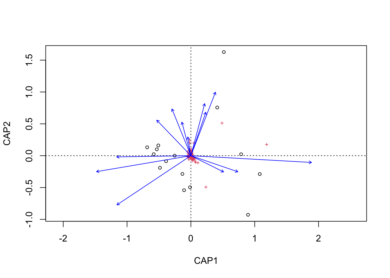
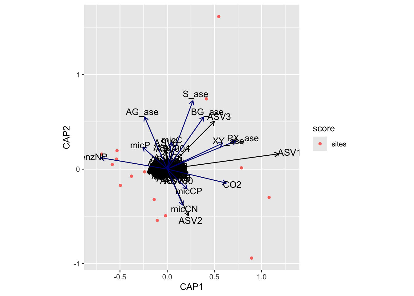
(16S rRNA) Figure 7 | Distance-based Redundancy Analysis (db-RDA) of PIME filtered data based on Bray-Curtis dissimilarity showing the relationships between community composition change versus edaphic properties.

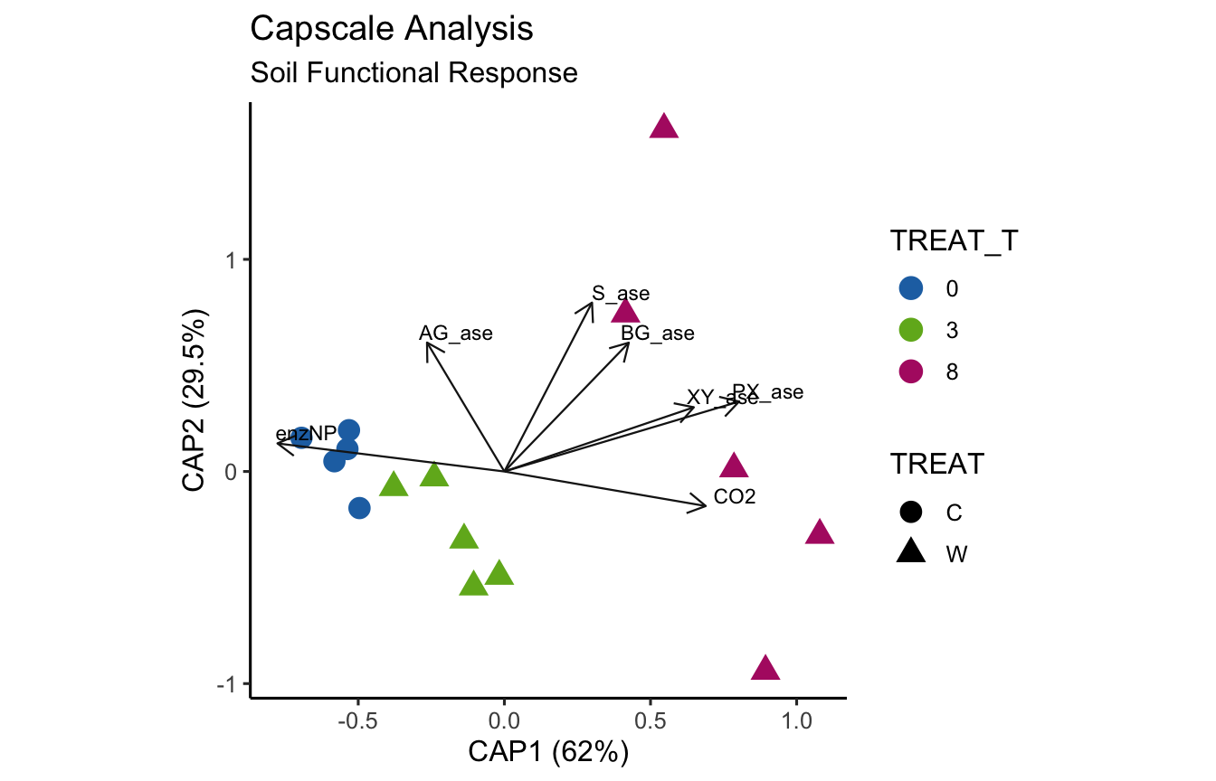
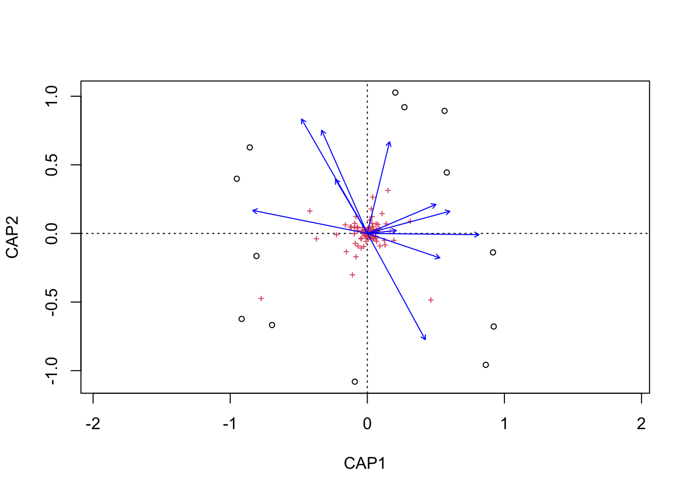
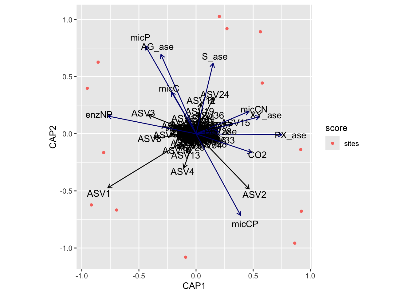
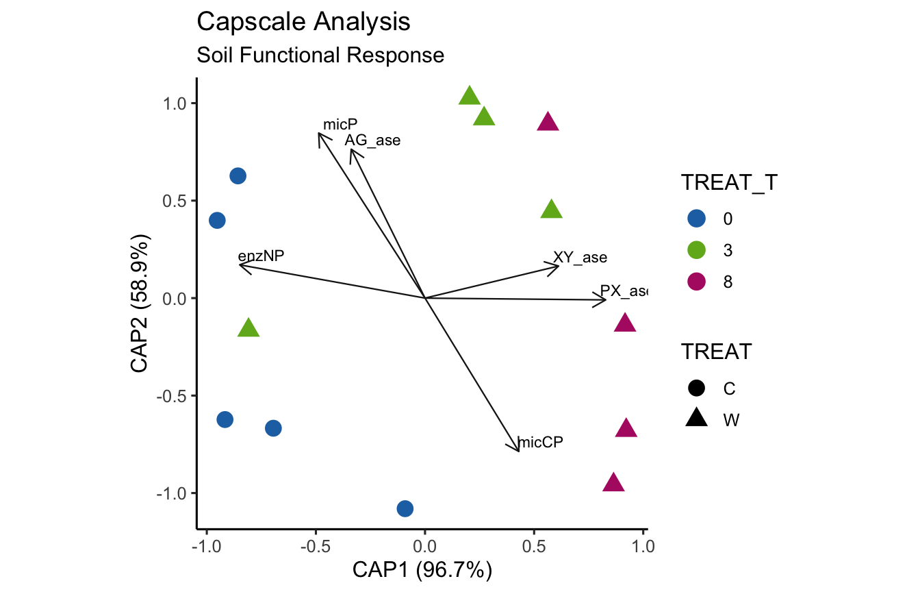
(16S rRNA) Figure 8 | Distance-based Redundancy Analysis (db-RDA) of PIME filtered data based on Bray-Curtis dissimilarity showing the relationships between community composition change versus microbial functional response.

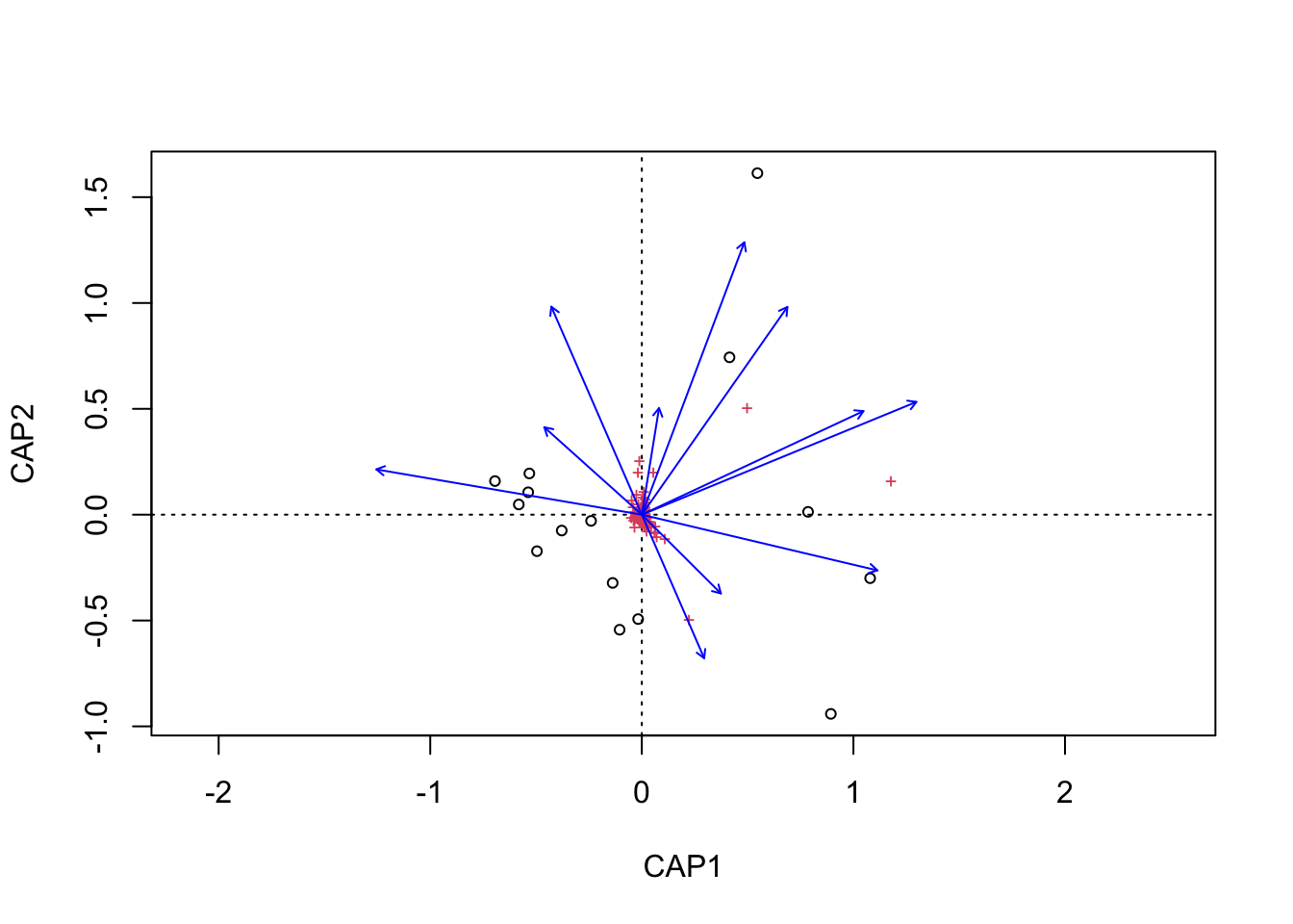
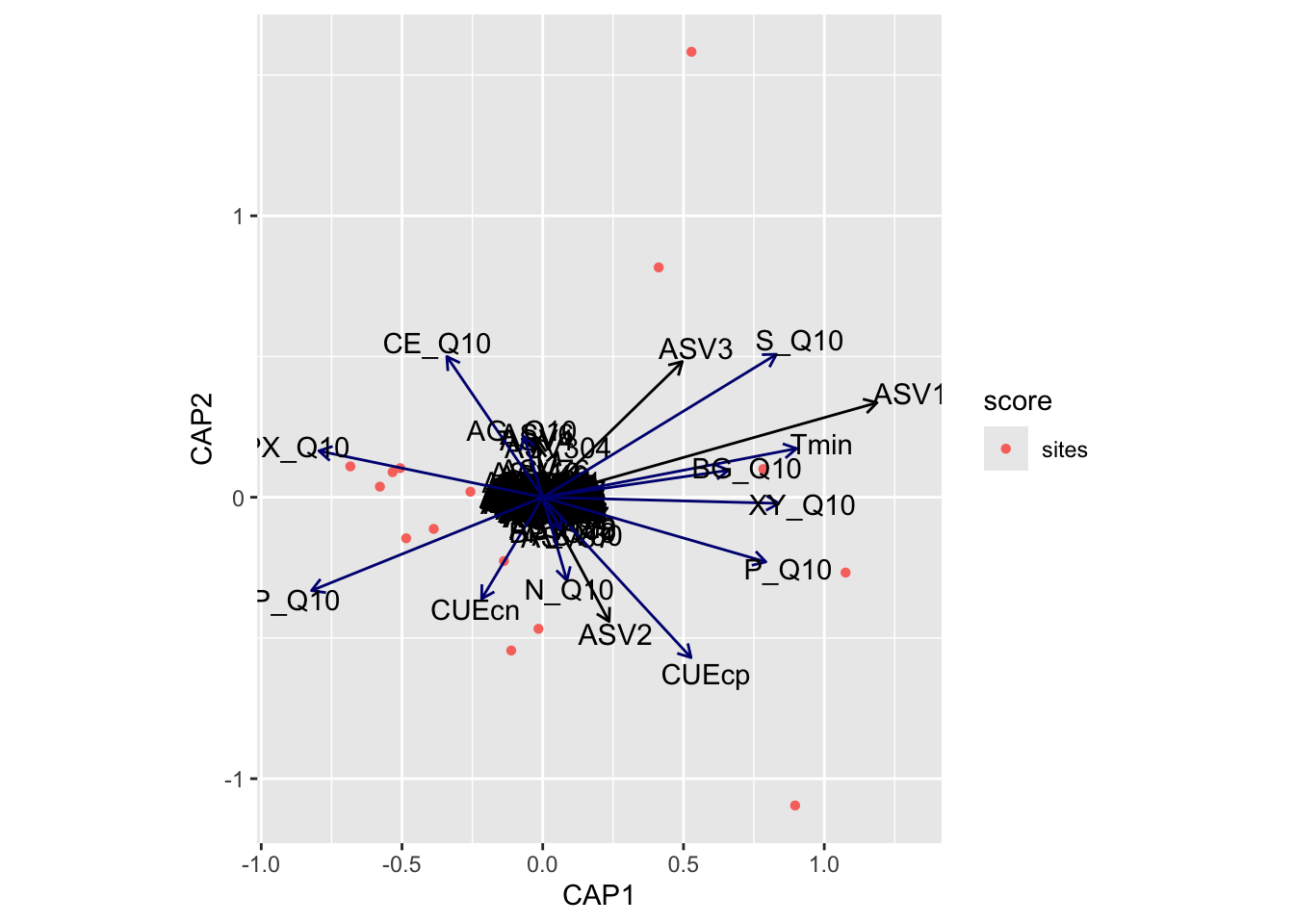
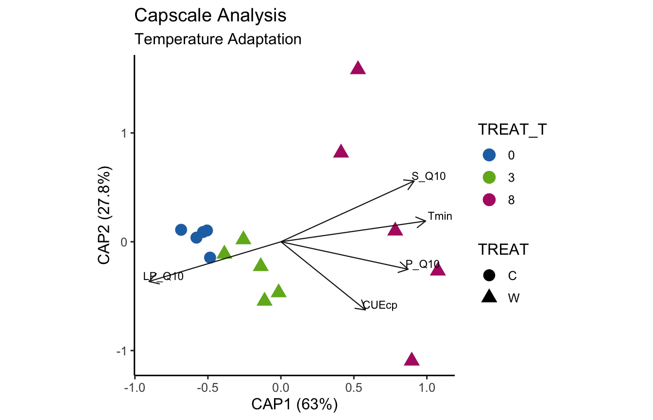
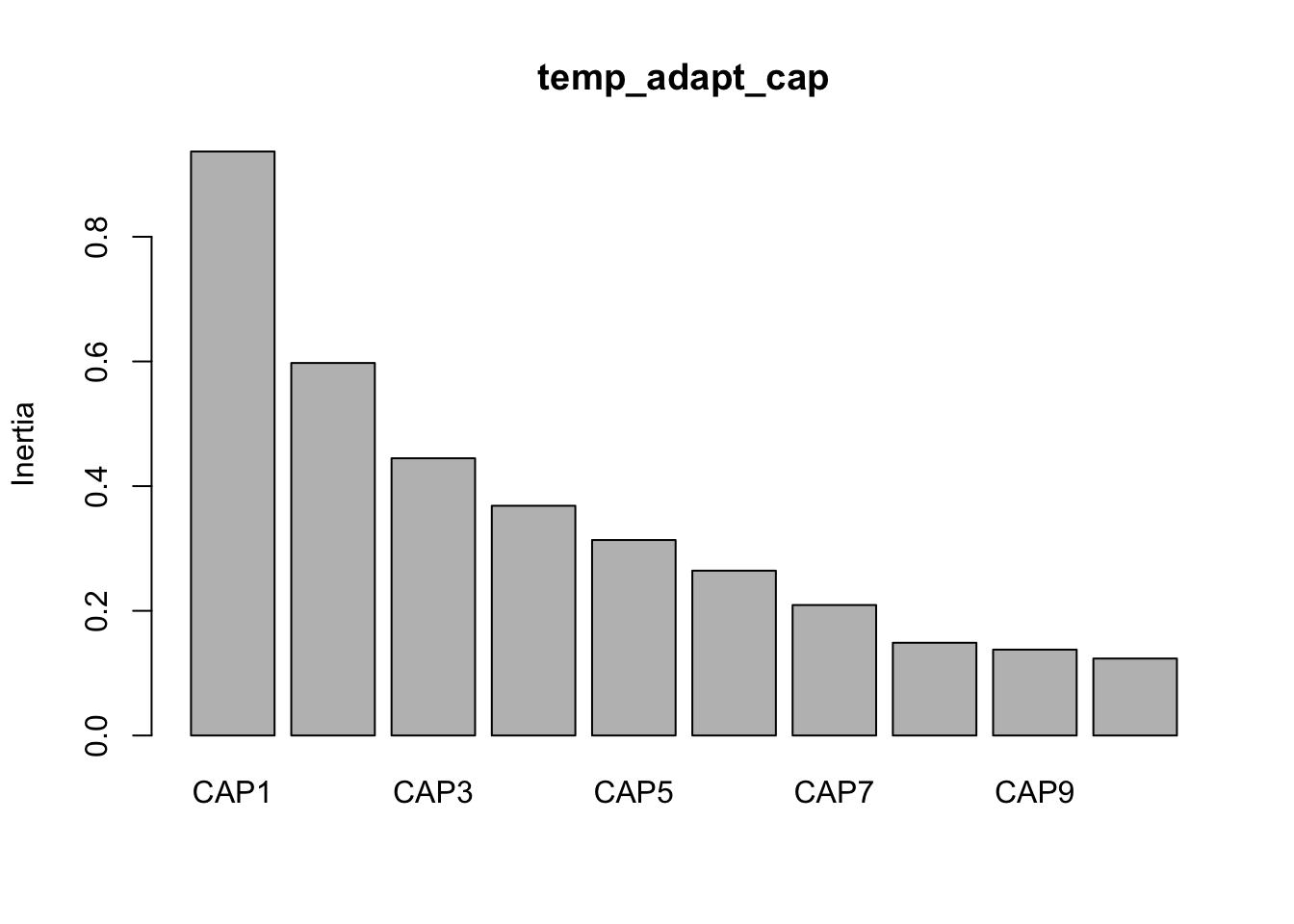
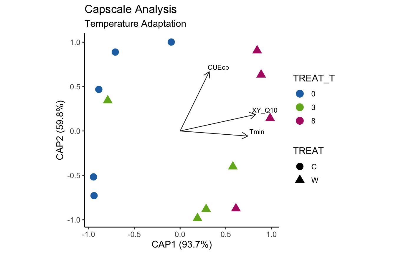
(16S rRNA) Figure 9 | Distance-based Redundancy Analysis (db-RDA) of PIME filtered data based on Bray-Curtis dissimilarity showing the relationships between community composition change versus temperature adaptation.

ITS

Data Formating

Transform ps Objects

The first step is to transform the phyloseq objects.

Show the code

samp_ps <- c("its18_ps_work", "its18_ps_pime", "its18_ps_perfect", 
             "its18_ps_work_otu", "its18_ps_pime_otu", "its18_ps_perfect_otu")
for (i in samp_ps) {
     tmp_get <- get(i)
     tmp_ps <- transform_sample_counts(tmp_get, function(otu) 1e5 * otu/sum(otu))
     tmp_ps@phy_tree <- NULL
     tmp_ps <- prune_samples(sample_sums(tmp_ps) > 0, tmp_ps)
     tmp_samp <- data.frame(sample_data(tmp_get))
     tmp_samp <- tmp_samp %>% dplyr::rename("TREAT_T" = "TEMP")
     tmp_ps <- merge_phyloseq(tmp_ps, sample_data)
     sample_data(tmp_ps) <- tmp_samp
     tmp_name <- purrr::map_chr(i, ~ paste0(., "_prop"))
     print(tmp_name)
     assign(tmp_name, tmp_ps)
     rm(list = ls(pattern = "tmp_"))
}

Format for mctoolsr

Then a bit of formatting to make the data compatible with mctoolsr.

Show the code

for (i in samp_ps) {
     tmp_get <- get(purrr::map_chr(i, ~ paste0(., "_prop")))
     tmp_tax <- data.frame(tax_table(tmp_get))
     tmp_tax$ASV_SEQ <- NULL
     
     tmp_col_names <- colnames(tmp_tax)
     tmp_tax_merge <- tmp_tax %>% tidyr::unite(taxonomy, 
                                               all_of(tmp_col_names), 
                                               sep = ";")
     tmp_tax_merge <- tmp_tax_merge %>% tibble::rownames_to_column("#OTU_ID")
     tmp_otu <- data.frame(t(otu_table(tmp_get)))
     tmp_otu <- tmp_otu %>% tibble::rownames_to_column("#OTU_ID")
     tmp_otu_tax <- dplyr::left_join(tmp_otu, tmp_tax_merge, by = "#OTU_ID")

     tmp_samp <- data.frame(sample_data(tmp_get))
     tmp_samp[,c(1,3)] <- NULL
     tmp_samp <- tmp_samp %>% tibble::rownames_to_column("#SampleID")

     tmp_metad <- metad %>% dplyr::rename("#SampleID" = "id")
     tmp_metad[,2:5] <- NULL
     tmp_md <- dplyr::left_join(tmp_samp, tmp_metad, by = "#SampleID")
     
     tmp_otu_name <- purrr::map_chr(i, ~ paste0(., "_otu_tax"))
     print(tmp_otu_name)
     assign(tmp_otu_name, tmp_otu_tax)

     tmp_md_name <- purrr::map_chr(i, ~ paste0(., "_md"))
     print(tmp_md_name)
     assign(tmp_md_name, tmp_md)

     tmp_path <- file.path("files/metadata/tables/")
     write_delim(tmp_otu_tax, paste(tmp_path, tmp_otu_name, ".txt", sep = ""), delim = "\t")
     write_delim(tmp_md, paste(tmp_path, tmp_md_name, ".txt", sep = ""), delim = "\t")
     rm(list = ls(pattern = "tmp_"))
}

Show the code

for (i in samp_ps) {
     tmp_path <- file.path("files/metadata/tables/")
     tmp_otu_name <- purrr::map_chr(i, ~ paste0(., "_otu_tax"))
     tmp_md_name <- purrr::map_chr(i, ~ paste0(., "_md"))
     tmp_tax_table_fp <- paste(tmp_path, tmp_otu_name, ".txt", sep = "")
     tmp_map_fp <- paste(tmp_path, tmp_md_name, ".txt", sep = "")
     tmp_input <- load_taxa_table(tmp_tax_table_fp, tmp_map_fp)
     tmp_input_name <- purrr::map_chr(i, ~ paste0(., "_mc"))
     print(tmp_input_name)
     assign(tmp_input_name, tmp_input)
     rm(list = ls(pattern = "tmp_"))
}
rm(list = ls(pattern = "_md"))
rm(list = ls(pattern = "_otu_tax"))

Choose Data Set

At this point in the code we need to choose a data set to use, formatted with mctoolsr. Remember, there are four choices:

Complete ASV data set.
Arbitrary filtered ASV data set.
PERfect filtered ASV data set.
PIME filtered ASV data set.

This way, if we want to test other data sets we only need to change the name here.

objects(pattern = "_mc")
its18_select_mc <- its18_ps_pime_mc

Normality Tests

Show the code

temp_md <- its18_select_mc$map_loaded
temp_md[,1:9] <- NULL
shap_results <- NULL

for (i in colnames(temp_md)) {
  tmp_shap <- shapiro.test(temp_md[[i]])
  tmp_p <- round(tmp_shap$p.value, digits = 5)
  tmp_res <- eval(isTRUE(tmp_shap$p.value < 0.05))
  shap_results <- rbind(shap_results, data.frame(i, tmp_p, tmp_res))
  rm(list = ls(pattern = "tmp_"))
}
colnames(shap_results) <- c("parameter", "p-value", "tranform")
shap_results
dplyr::filter(shap_results, tranform == "TRUE")
md_to_tranform <- shap_results$parameter[shap_results$tranform == TRUE]
rm(list = ls(pattern = "temp_md"))

Show the results of each normality test for metadata parameters

(ITS) Table 2 | Results of the Shapiro-Wilk Normality Tests. P-values in red are significance (p-value < 0.05) meaning the parameter needs to be normalized.

Looks like we need to transform 21 metadata parameters.

Normalize Parameters

Here we use the R package bestNormalize to find and execute the best normalizing transformation. The function will test the following normalizing transformations:

arcsinh_x performs an arcsinh transformation.
boxcox Perform a Box-Cox transformation and center/scale a vector to attempt normalization. boxcox estimates the optimal value of lambda for the Box-Cox transformation. The function will return an error if a user attempt to transform nonpositive data.
yeojohnson Perform a Yeo-Johnson Transformation and center/scale a vector to attempt normalization. yeojohnson estimates the optimal value of lambda for the Yeo-Johnson transformation. The Yeo-Johnson is similar to the Box-Cox method, however it allows for the transformation of nonpositive data as well.
orderNorm The Ordered Quantile (ORQ) normalization transformation, orderNorm(), is a rank-based procedure by which the values of a vector are mapped to their percentile, which is then mapped to the same percentile of the normal distribution. Without the presence of ties, this essentially guarantees that the transformation leads to a uniform distribution.
log_x performs a simple log transformation. The parameter a is essentially estimated by the training set by default (estimated as the minimum possible to some extent epsilon), while the base must be specified beforehand. The default base of the log is 10.
sqrt_x performs a simple square-root transformation. The parameter a is essentially estimated by the training set by default (estimated as the minimum possible), while the base must be specified beforehand.
exp_x performs a simple exponential transformation.

Show the code

set.seed(119)

for (i in md_to_tranform) {
  tmp_md <- its18_select_mc$map_loaded
  tmp_best_norm <- bestNormalize(tmp_md[[i]], r = 1, k = 5, loo = TRUE)
  tmp_name <- purrr::map_chr(i, ~ paste0(., "_best_norm_test"))
  assign(tmp_name, tmp_best_norm)
  print(tmp_name)
  rm(list = ls(pattern = "tmp_"))
}

Show the chosen transformations


## bestNormalize Chosen transformation of AST ## 
orderNorm Transformation with 13 nonmissing obs and no ties 
 - Original quantiles:
   0%   25%   50%   75%  100% 
25.80 26.26 28.80 29.90 41.77 
_____________________________________

## bestNormalize Chosen transformation of H2O ## 
orderNorm Transformation with 13 nonmissing obs and no ties 
 - Original quantiles:
   0%   25%   50%   75%  100% 
0.204 0.261 0.377 0.385 0.401 
_____________________________________

## bestNormalize Chosen transformation of Al ## 
Standardized asinh(x) Transformation with 13 nonmissing obs.:
 Relevant statistics:
 - mean (before standardization) = 0.005384372 
 - sd (before standardization) = 0.007762057 
_____________________________________

## bestNormalize Chosen transformation of Fe ## 
Standardized asinh(x) Transformation with 13 nonmissing obs.:
 Relevant statistics:
 - mean (before standardization) = 0.01076821 
 - sd (before standardization) = 0.0103749 
_____________________________________

## bestNormalize Chosen transformation of TEB ## 
orderNorm Transformation with 13 nonmissing obs and ties
 - 10 unique values 
 - Original quantiles:
  0%  25%  50%  75% 100% 
41.6 43.3 45.1 48.7 61.7 
_____________________________________

## bestNormalize Chosen transformation of ECEC ## 
orderNorm Transformation with 13 nonmissing obs and ties
 - 10 unique values 
 - Original quantiles:
  0%  25%  50%  75% 100% 
41.7 43.3 45.3 48.8 61.8 
_____________________________________

## bestNormalize Chosen transformation of minNO3 ## 
orderNorm Transformation with 13 nonmissing obs and no ties 
 - Original quantiles:
    0%    25%    50%    75%   100% 
 11.31  19.67  22.71  37.33 106.42 
_____________________________________

## bestNormalize Chosen transformation of minTIN ## 
orderNorm Transformation with 13 nonmissing obs and ties
 - 12 unique values 
 - Original quantiles:
    0%    25%    50%    75%   100% 
 12.96  21.50  23.99  42.08 110.75 
_____________________________________

## bestNormalize Chosen transformation of DOC ## 
orderNorm Transformation with 13 nonmissing obs and no ties 
 - Original quantiles:
    0%    25%    50%    75%   100% 
 33.20  44.30  56.68  63.79 118.74 
_____________________________________

## bestNormalize Chosen transformation of BG_ase ## 
orderNorm Transformation with 13 nonmissing obs and no ties 
 - Original quantiles:
  0%  25%  50%  75% 100% 
3.04 3.92 4.22 4.62 9.09 
_____________________________________

## bestNormalize Chosen transformation of BP_ase ## 
orderNorm Transformation with 13 nonmissing obs and no ties 
 - Original quantiles:
  0%  25%  50%  75% 100% 
1.77 2.33 3.02 3.50 7.28 
_____________________________________

## bestNormalize Chosen transformation of P_ase ## 
Standardized Box Cox Transformation with 13 nonmissing obs.:
 Estimated statistics:
 - lambda = -0.9999576 
 - mean (before standardization) = 0.9480149 
 - sd (before standardization) = 0.01593697 
_____________________________________

## bestNormalize Chosen transformation of N_ase ## 
orderNorm Transformation with 13 nonmissing obs and no ties 
 - Original quantiles:
  0%  25%  50%  75% 100% 
2.57 2.95 3.58 4.52 8.34 
_____________________________________

## bestNormalize Chosen transformation of XY_ase ## 
orderNorm Transformation with 13 nonmissing obs and ties
 - 11 unique values 
 - Original quantiles:
  0%  25%  50%  75% 100% 
0.66 0.76 1.11 1.36 2.52 
_____________________________________

## bestNormalize Chosen transformation of BG_Q10 ## 
orderNorm Transformation with 13 nonmissing obs and ties
 - 11 unique values 
 - Original quantiles:
  0%  25%  50%  75% 100% 
1.31 1.36 1.39 1.56 1.76 
_____________________________________

## bestNormalize Chosen transformation of CE_Q10 ## 
orderNorm Transformation with 13 nonmissing obs and ties
 - 12 unique values 
 - Original quantiles:
  0%  25%  50%  75% 100% 
1.76 1.87 1.95 2.00 2.36 
_____________________________________

## bestNormalize Chosen transformation of CO2 ## 
Standardized asinh(x) Transformation with 13 nonmissing obs.:
 Relevant statistics:
 - mean (before standardization) = 2.626573 
 - sd (before standardization) = 0.7396036 
_____________________________________

## bestNormalize Chosen transformation of PX_ase ## 
orderNorm Transformation with 13 nonmissing obs and no ties 
 - Original quantiles:
    0%    25%    50%    75%   100% 
 81.25  94.13 119.75 211.18 294.39 
_____________________________________

## bestNormalize Chosen transformation of PX_Q10 ## 
Standardized Yeo-Johnson Transformation with 13 nonmissing obs.:
 Estimated statistics:
 - lambda = -4.999963 
 - mean (before standardization) = 0.1968145 
 - sd (before standardization) = 0.001394949 
_____________________________________

## bestNormalize Chosen transformation of CUEcp ## 
orderNorm Transformation with 13 nonmissing obs and ties
 - 9 unique values 
 - Original quantiles:
  0%  25%  50%  75% 100% 
0.15 0.17 0.19 0.21 0.33 
_____________________________________

## bestNormalize Chosen transformation of PUE ## 
orderNorm Transformation with 13 nonmissing obs and ties
 - 6 unique values 
 - Original quantiles:
  0%  25%  50%  75% 100% 
0.77 0.88 0.90 0.91 0.92 
_____________________________________

Show the complete bestNormalize results


## Results of bestNormalize for AST ## 
Best Normalizing transformation with 13 Observations
 Estimated Normality Statistics (Pearson P / df, lower => more normal):
 - arcsinh(x): 3.2051
 - Box-Cox: 3.2051
 - Center+scale: 4.1282
 - Exp(x): 17.9744
 - Log_b(x+a): 3.2051
 - orderNorm (ORQ): 0.1282
 - sqrt(x + a): 4.1282
 - Yeo-Johnson: 2.2821
Estimation method: Out-of-sample via leave-one-out CV
 
Based off these, bestNormalize chose:
orderNorm Transformation with 13 nonmissing obs and no ties 
 - Original quantiles:
   0%   25%   50%   75%  100% 
25.80 26.26 28.80 29.90 41.77 
_____________________________________

## Results of bestNormalize for H2O ## 
Best Normalizing transformation with 13 Observations
 Estimated Normality Statistics (Pearson P / df, lower => more normal):
 - arcsinh(x): 7.2051
 - Box-Cox: 6.2821
 - Center+scale: 8.1282
 - Exp(x): 6.2821
 - Log_b(x+a): 7.2051
 - orderNorm (ORQ): 0.4359
 - sqrt(x + a): 7.2051
 - Yeo-Johnson: 6.2821
Estimation method: Out-of-sample via leave-one-out CV
 
Based off these, bestNormalize chose:
orderNorm Transformation with 13 nonmissing obs and no ties 
 - Original quantiles:
   0%   25%   50%   75%  100% 
0.204 0.261 0.377 0.385 0.401 
_____________________________________

## Results of bestNormalize for Al ## 
Best Normalizing transformation with 13 Observations
 Estimated Normality Statistics (Pearson P / df, lower => more normal):
 - arcsinh(x): 7.5128
 - Center+scale: 7.5128
 - Exp(x): 7.5128
 - Log_b(x+a): 9.359
 - orderNorm (ORQ): 7.5128
 - sqrt(x + a): 7.5128
 - Yeo-Johnson: 7.5128
Estimation method: Out-of-sample via leave-one-out CV
 
Based off these, bestNormalize chose:
Standardized asinh(x) Transformation with 13 nonmissing obs.:
 Relevant statistics:
 - mean (before standardization) = 0.005384372 
 - sd (before standardization) = 0.007762057 
_____________________________________

## Results of bestNormalize for Fe ## 
Best Normalizing transformation with 13 Observations
 Estimated Normality Statistics (Pearson P / df, lower => more normal):
 - arcsinh(x): 7.2051
 - Center+scale: 7.2051
 - Exp(x): 7.2051
 - Log_b(x+a): 7.2051
 - orderNorm (ORQ): 7.2051
 - sqrt(x + a): 7.2051
 - Yeo-Johnson: 7.2051
Estimation method: Out-of-sample via leave-one-out CV
 
Based off these, bestNormalize chose:
Standardized asinh(x) Transformation with 13 nonmissing obs.:
 Relevant statistics:
 - mean (before standardization) = 0.01076821 
 - sd (before standardization) = 0.0103749 
_____________________________________

## Results of bestNormalize for TEB ## 
Best Normalizing transformation with 13 Observations
 Estimated Normality Statistics (Pearson P / df, lower => more normal):
 - arcsinh(x): 1.6667
 - Box-Cox: 1.6667
 - Center+scale: 4.7436
 - Exp(x): 17.9744
 - Log_b(x+a): 1.6667
 - orderNorm (ORQ): 0.4359
 - sqrt(x + a): 3.2051
 - Yeo-Johnson: 1.359
Estimation method: Out-of-sample via leave-one-out CV
 
Based off these, bestNormalize chose:
orderNorm Transformation with 13 nonmissing obs and ties
 - 10 unique values 
 - Original quantiles:
  0%  25%  50%  75% 100% 
41.6 43.3 45.1 48.7 61.7 
_____________________________________

## Results of bestNormalize for ECEC ## 
Best Normalizing transformation with 13 Observations
 Estimated Normality Statistics (Pearson P / df, lower => more normal):
 - arcsinh(x): 1.6667
 - Box-Cox: 1.6667
 - Center+scale: 3.2051
 - Exp(x): 17.9744
 - Log_b(x+a): 1.6667
 - orderNorm (ORQ): 0.4359
 - sqrt(x + a): 3.2051
 - Yeo-Johnson: 1.359
Estimation method: Out-of-sample via leave-one-out CV
 
Based off these, bestNormalize chose:
orderNorm Transformation with 13 nonmissing obs and ties
 - 10 unique values 
 - Original quantiles:
  0%  25%  50%  75% 100% 
41.7 43.3 45.3 48.8 61.8 
_____________________________________

## Results of bestNormalize for minNO3 ## 
Best Normalizing transformation with 13 Observations
 Estimated Normality Statistics (Pearson P / df, lower => more normal):
 - arcsinh(x): 3.5128
 - Box-Cox: 3.5128
 - Center+scale: 5.359
 - Exp(x): 17.9744
 - Log_b(x+a): 3.5128
 - orderNorm (ORQ): 0.7436
 - sqrt(x + a): 2.5897
 - Yeo-Johnson: 3.5128
Estimation method: Out-of-sample via leave-one-out CV
 
Based off these, bestNormalize chose:
orderNorm Transformation with 13 nonmissing obs and no ties 
 - Original quantiles:
    0%    25%    50%    75%   100% 
 11.31  19.67  22.71  37.33 106.42 
_____________________________________

## Results of bestNormalize for minTIN ## 
Best Normalizing transformation with 13 Observations
 Estimated Normality Statistics (Pearson P / df, lower => more normal):
 - arcsinh(x): 1.359
 - Box-Cox: 2.2821
 - Center+scale: 4.1282
 - Exp(x): 17.9744
 - Log_b(x+a): 1.359
 - orderNorm (ORQ): 0.7436
 - sqrt(x + a): 2.2821
 - Yeo-Johnson: 2.2821
Estimation method: Out-of-sample via leave-one-out CV
 
Based off these, bestNormalize chose:
orderNorm Transformation with 13 nonmissing obs and ties
 - 12 unique values 
 - Original quantiles:
    0%    25%    50%    75%   100% 
 12.96  21.50  23.99  42.08 110.75 
_____________________________________

## Results of bestNormalize for DOC ## 
Best Normalizing transformation with 13 Observations
 Estimated Normality Statistics (Pearson P / df, lower => more normal):
 - arcsinh(x): 2.8974
 - Box-Cox: 2.8974
 - Center+scale: 3.5128
 - Exp(x): 17.9744
 - Log_b(x+a): 2.8974
 - orderNorm (ORQ): 0.4359
 - sqrt(x + a): 1.9744
 - Yeo-Johnson: 2.8974
Estimation method: Out-of-sample via leave-one-out CV
 
Based off these, bestNormalize chose:
orderNorm Transformation with 13 nonmissing obs and no ties 
 - Original quantiles:
    0%    25%    50%    75%   100% 
 33.20  44.30  56.68  63.79 118.74 
_____________________________________

## Results of bestNormalize for BG_ase ## 
Best Normalizing transformation with 13 Observations
 Estimated Normality Statistics (Pearson P / df, lower => more normal):
 - arcsinh(x): 3.8205
 - Box-Cox: 2.2821
 - Center+scale: 4.1282
 - Exp(x): 14.8974
 - Log_b(x+a): 3.8205
 - orderNorm (ORQ): 0.4359
 - sqrt(x + a): 3.5128
 - Yeo-Johnson: 1.6667
Estimation method: Out-of-sample via leave-one-out CV
 
Based off these, bestNormalize chose:
orderNorm Transformation with 13 nonmissing obs and no ties 
 - Original quantiles:
  0%  25%  50%  75% 100% 
3.04 3.92 4.22 4.62 9.09 
_____________________________________

## Results of bestNormalize for BP_ase ## 
Best Normalizing transformation with 13 Observations
 Estimated Normality Statistics (Pearson P / df, lower => more normal):
 - arcsinh(x): 1.6667
 - Box-Cox: 1.6667
 - Center+scale: 4.1282
 - Exp(x): 5.6667
 - Log_b(x+a): 1.6667
 - orderNorm (ORQ): 0.4359
 - sqrt(x + a): 1.6667
 - Yeo-Johnson: 1.6667
Estimation method: Out-of-sample via leave-one-out CV
 
Based off these, bestNormalize chose:
orderNorm Transformation with 13 nonmissing obs and no ties 
 - Original quantiles:
  0%  25%  50%  75% 100% 
1.77 2.33 3.02 3.50 7.28 
_____________________________________

## Results of bestNormalize for P_ase ## 
Best Normalizing transformation with 13 Observations
 Estimated Normality Statistics (Pearson P / df, lower => more normal):
 - arcsinh(x): 1.6667
 - Box-Cox: 0.4359
 - Center+scale: 3.2051
 - Exp(x): 17.9744
 - Log_b(x+a): 1.6667
 - orderNorm (ORQ): 0.4359
 - sqrt(x + a): 1.9744
 - Yeo-Johnson: 0.4359
Estimation method: Out-of-sample via leave-one-out CV
 
Based off these, bestNormalize chose:
Standardized Box Cox Transformation with 13 nonmissing obs.:
 Estimated statistics:
 - lambda = -0.9999576 
 - mean (before standardization) = 0.9480149 
 - sd (before standardization) = 0.01593697 
_____________________________________

## Results of bestNormalize for N_ase ## 
Best Normalizing transformation with 13 Observations
 Estimated Normality Statistics (Pearson P / df, lower => more normal):
 - arcsinh(x): 1.9744
 - Box-Cox: 2.2821
 - Center+scale: 2.8974
 - Exp(x): 17.9744
 - Log_b(x+a): 1.9744
 - orderNorm (ORQ): 0.4359
 - sqrt(x + a): 2.8974
 - Yeo-Johnson: 0.4359
Estimation method: Out-of-sample via leave-one-out CV
 
Based off these, bestNormalize chose:
orderNorm Transformation with 13 nonmissing obs and no ties 
 - Original quantiles:
  0%  25%  50%  75% 100% 
2.57 2.95 3.58 4.52 8.34 
_____________________________________

## Results of bestNormalize for XY_ase ## 
Best Normalizing transformation with 13 Observations
 Estimated Normality Statistics (Pearson P / df, lower => more normal):
 - arcsinh(x): 1.0513
 - Box-Cox: 0.4359
 - Center+scale: 2.8974
 - Exp(x): 9.0513
 - Log_b(x+a): 1.0513
 - orderNorm (ORQ): 0.1282
 - sqrt(x + a): 1.359
 - Yeo-Johnson: 0.4359
Estimation method: Out-of-sample via leave-one-out CV
 
Based off these, bestNormalize chose:
orderNorm Transformation with 13 nonmissing obs and ties
 - 11 unique values 
 - Original quantiles:
  0%  25%  50%  75% 100% 
0.66 0.76 1.11 1.36 2.52 
_____________________________________

## Results of bestNormalize for BG_Q10 ## 
Best Normalizing transformation with 13 Observations
 Estimated Normality Statistics (Pearson P / df, lower => more normal):
 - arcsinh(x): 1.9744
 - Box-Cox: 1.9744
 - Center+scale: 2.2821
 - Exp(x): 5.359
 - Log_b(x+a): 1.9744
 - orderNorm (ORQ): 0.4359
 - sqrt(x + a): 1.9744
 - Yeo-Johnson: 1.9744
Estimation method: Out-of-sample via leave-one-out CV
 
Based off these, bestNormalize chose:
orderNorm Transformation with 13 nonmissing obs and ties
 - 11 unique values 
 - Original quantiles:
  0%  25%  50%  75% 100% 
1.31 1.36 1.39 1.56 1.76 
_____________________________________

## Results of bestNormalize for CE_Q10 ## 
Best Normalizing transformation with 13 Observations
 Estimated Normality Statistics (Pearson P / df, lower => more normal):
 - arcsinh(x): 1.6667
 - Box-Cox: 1.6667
 - Center+scale: 1.6667
 - Exp(x): 4.1282
 - Log_b(x+a): 1.6667
 - orderNorm (ORQ): 0.4359
 - sqrt(x + a): 1.6667
 - Yeo-Johnson: 0.7436
Estimation method: Out-of-sample via leave-one-out CV
 
Based off these, bestNormalize chose:
orderNorm Transformation with 13 nonmissing obs and ties
 - 12 unique values 
 - Original quantiles:
  0%  25%  50%  75% 100% 
1.76 1.87 1.95 2.00 2.36 
_____________________________________

## Results of bestNormalize for CO2 ## 
Best Normalizing transformation with 13 Observations
 Estimated Normality Statistics (Pearson P / df, lower => more normal):
 - arcsinh(x): 1.0513
 - Box-Cox: 3.5128
 - Center+scale: 11.5128
 - Exp(x): 17.9744
 - Log_b(x+a): 1.0513
 - orderNorm (ORQ): 1.0513
 - sqrt(x + a): 2.8974
 - Yeo-Johnson: 1.9744
Estimation method: Out-of-sample via leave-one-out CV
 
Based off these, bestNormalize chose:
Standardized asinh(x) Transformation with 13 nonmissing obs.:
 Relevant statistics:
 - mean (before standardization) = 2.626573 
 - sd (before standardization) = 0.7396036 
_____________________________________

## Results of bestNormalize for PX_ase ## 
Best Normalizing transformation with 13 Observations
 Estimated Normality Statistics (Pearson P / df, lower => more normal):
 - arcsinh(x): 1.9744
 - Box-Cox: 2.2821
 - Center+scale: 4.1282
 - Exp(x): 17.9744
 - Log_b(x+a): 1.9744
 - orderNorm (ORQ): 0.4359
 - sqrt(x + a): 1.9744
 - Yeo-Johnson: 2.2821
Estimation method: Out-of-sample via leave-one-out CV
 
Based off these, bestNormalize chose:
orderNorm Transformation with 13 nonmissing obs and no ties 
 - Original quantiles:
    0%    25%    50%    75%   100% 
 81.25  94.13 119.75 211.18 294.39 
_____________________________________

## Results of bestNormalize for PX_Q10 ## 
Best Normalizing transformation with 13 Observations
 Estimated Normality Statistics (Pearson P / df, lower => more normal):
 - arcsinh(x): 14.5897
 - Box-Cox: 3.2051
 - Center+scale: 17.9744
 - Exp(x): 17.9744
 - Log_b(x+a): 11.5128
 - orderNorm (ORQ): 2.2821
 - sqrt(x + a): 17.9744
 - Yeo-Johnson: 1.0513
Estimation method: Out-of-sample via leave-one-out CV
 
Based off these, bestNormalize chose:
Standardized Yeo-Johnson Transformation with 13 nonmissing obs.:
 Estimated statistics:
 - lambda = -4.999963 
 - mean (before standardization) = 0.1968145 
 - sd (before standardization) = 0.001394949 
_____________________________________

## Results of bestNormalize for CUEcp ## 
Best Normalizing transformation with 13 Observations
 Estimated Normality Statistics (Pearson P / df, lower => more normal):
 - arcsinh(x): 3.5128
 - Box-Cox: 1.359
 - Center+scale: 3.5128
 - Exp(x): 4.4359
 - Log_b(x+a): 1.359
 - orderNorm (ORQ): 0.7436
 - sqrt(x + a): 3.5128
 - Yeo-Johnson: 2.5897
Estimation method: Out-of-sample via leave-one-out CV
 
Based off these, bestNormalize chose:
orderNorm Transformation with 13 nonmissing obs and ties
 - 9 unique values 
 - Original quantiles:
  0%  25%  50%  75% 100% 
0.15 0.17 0.19 0.21 0.33 
_____________________________________

## Results of bestNormalize for PUE ## 
Best Normalizing transformation with 13 Observations
 Estimated Normality Statistics (Pearson P / df, lower => more normal):
 - arcsinh(x): 5.9744
 - Box-Cox: 7.2051
 - Center+scale: 5.9744
 - Exp(x): 5.9744
 - Log_b(x+a): 7.2051
 - orderNorm (ORQ): 2.5897
 - sqrt(x + a): 5.9744
 - Yeo-Johnson: 5.9744
Estimation method: Out-of-sample via leave-one-out CV
 
Based off these, bestNormalize chose:
orderNorm Transformation with 13 nonmissing obs and ties
 - 6 unique values 
 - Original quantiles:
  0%  25%  50%  75% 100% 
0.77 0.88 0.90 0.91 0.92 
_____________________________________

Great, now we can add the normalized transformed data back to our mctoolsr metadata file.

Show the code

its18_select_mc_norm <- its18_select_mc

for (i in md_to_tranform) {
      tmp_get <- get(purrr::map_chr(i, ~ paste0(i, "_best_norm_test")))
      tmp_new_data <- tmp_get$x.t
      its18_select_mc_norm$map_loaded[[i]] <- tmp_new_data
      rm(list = ls(pattern = "tmp_"))
}

And rerun the Shapiro Tests.

Show the code

temp_md_norm <- its18_select_mc_norm$map_loaded
temp_md_norm[,1:9] <- NULL
shap_results_norm <- NULL

for (i in colnames(temp_md_norm)) {
  tmp_shap <- shapiro.test(temp_md_norm[[i]])
  tmp_p <- round(tmp_shap$p.value, digits = 5)
  tmp_res <- eval(isTRUE(tmp_shap$p.value < 0.05))
  shap_results_norm <- rbind(shap_results_norm, data.frame(i, tmp_p, tmp_res))
  rm(list = ls(pattern = "tmp_"))
}
colnames(shap_results_norm) <- c("parameter", "p-value", "tranform")
shap_results_norm
rm(list = ls(pattern = "temp_md_norm"))

And check if there are any parameters that are still significant for the normality test.

shap_results$parameter[shap_results_norm$tranform == TRUE]

[1] "Al" "Fe"

Normalized Metadata

Finally, here is a new summary table that includes all of the normalized data.

(ITS) Table 3 | Results of bestNormalize function applied to each parameter.

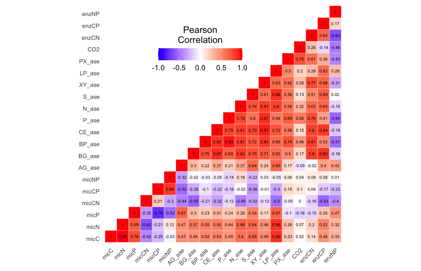
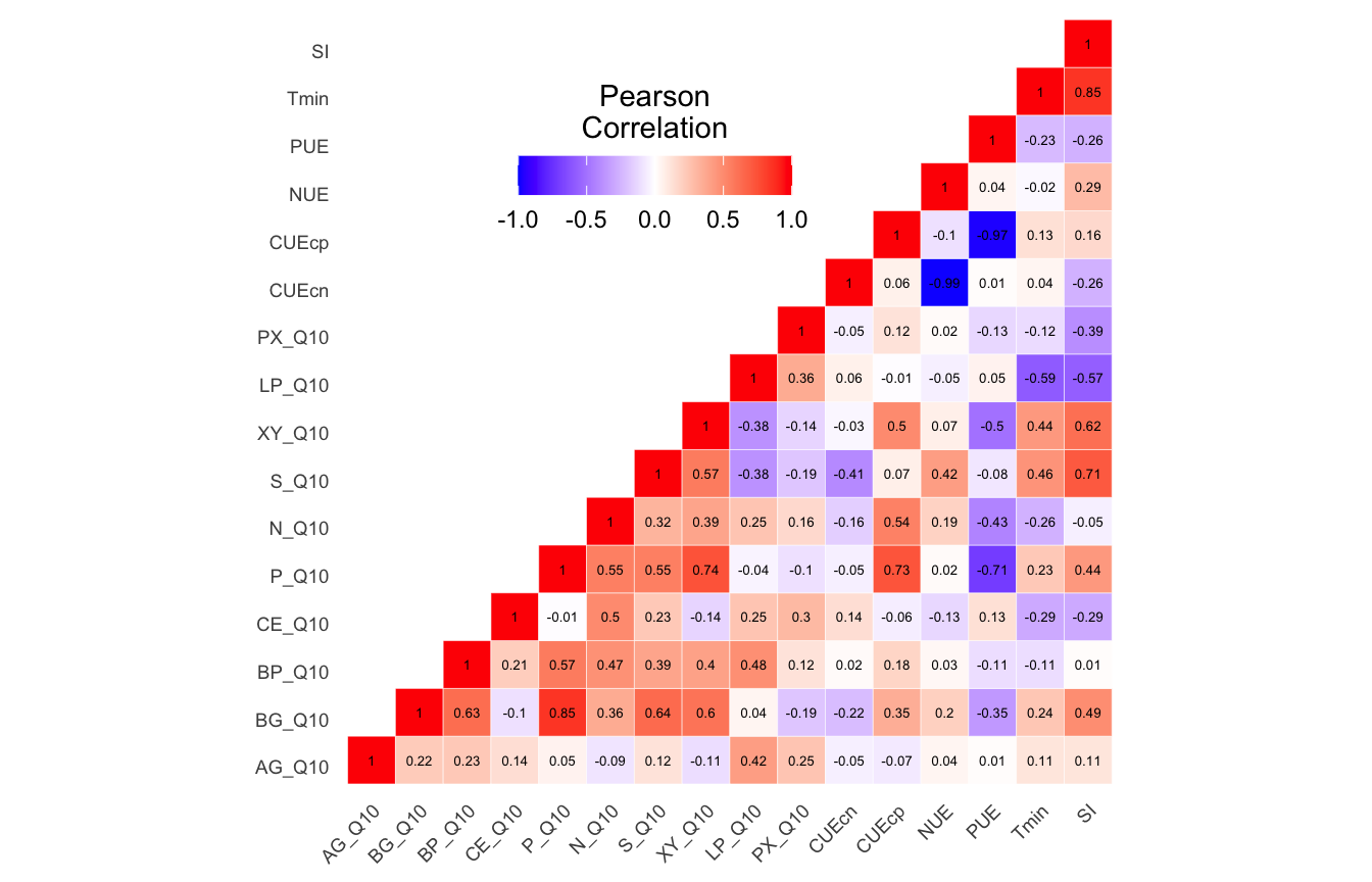
Autocorrelation Tests

Next, we test the metadata for autocorrelations. Do we do this on the original data or the transformed data? No idea, so let’s do both.

Split Metadata

We need to split the data into different groups.

Environmental and edaphic properties
Microbial functional responses
Temperature adaptation properties

We first create lists of metadata parameters.

Show the code

div <- c("PLOT", "TREAT", "TREAT_T", "PAIR", "Observed", "Shannon_exp", 
         "InvSimpson", "ATAP")

edaphic <- c("AST", "H2O", "N", "P", "Al", 
             "Ca", "Fe", "K", "Mg", "Mn", "Na", "TEB", "ECEC", "pH", 
             "NH4", "NO3", "PO4", "DOC", "DON", "DOCN")

soil_funct <- c("micC", "micN", "micP", "micCN", "micCP", "micNP", 
                "AG_ase", "BG_ase", "BP_ase", "CE_ase", "P_ase", "N_ase", 
                "S_ase", "XY_ase",  "LP_ase", "PX_ase", "CO2", 
                "enzCN", "enzCP", "enzNP")

temp_adapt <- c("AG_Q10", "BG_Q10", "BP_Q10", "CE_Q10", "P_Q10", "N_Q10", 
                "S_Q10", "XY_Q10", "LP_Q10", "PX_Q10", "CUEcn", "CUEcp", 
                "NUE", "PUE", "Tmin", "SI")

md_groups <- c("edaphic", "soil_funct", "temp_adapt")

# NoT uSed: minPO4, minNH4, minNO3, minTIN

And then use the lists to split the data sets by metadata group. Here, we do this for the original metadata and the metadata after normalization.

Show the code

select_md <- c("its18_select_mc", "its18_select_mc_norm")
for (i in select_md) {
   #tmp_get <- get(purrr::map_chr(i, ~ paste0(i, "_mc")))
   tmp_get <- get(i)
   tmp_md_all <- tmp_get$map_loaded
   tmp_div <- tmp_md_all %>% dplyr::select(all_of(div))
   tmp_div <- tmp_div %>% tibble::rownames_to_column("SampleID")
## edaphic      
   tmp_sub_edaphic <- tmp_md_all %>% dplyr::select(all_of(edaphic))
   tmp_sub_edaphic <- tmp_sub_edaphic %>% tibble::rownames_to_column("SampleID")
   tmp_edaphic <- dplyr::left_join(tmp_div, tmp_sub_edaphic, by = "SampleID")
   tmp_edaphic <- tmp_edaphic %>% tibble::column_to_rownames("SampleID")
## soil_funct
   tmp_sub_soil_funct <- tmp_md_all %>% dplyr::select(all_of(soil_funct))
   tmp_sub_soil_funct <- tmp_sub_soil_funct %>% tibble::rownames_to_column("SampleID")
   tmp_soil_funct <- dplyr::left_join(tmp_div, tmp_sub_soil_funct, by = "SampleID")
   tmp_soil_funct <- tmp_soil_funct %>% tibble::column_to_rownames("SampleID")      
## temp_adapt
   tmp_sub_temp_adapt <- tmp_md_all %>% dplyr::select(all_of(temp_adapt))
   tmp_sub_temp_adapt <- tmp_sub_temp_adapt %>% tibble::rownames_to_column("SampleID")
   tmp_temp_adapt <- dplyr::left_join(tmp_div, tmp_sub_temp_adapt, by = "SampleID")
   tmp_temp_adapt <- tmp_temp_adapt %>% tibble::column_to_rownames("SampleID")      
## combine
   tmp_list <- list(data_loaded = its18_select_mc$data_loaded, 
                    map_loaded = its18_select_mc$map_loaded, 
                    taxonomy_loaded = its18_select_mc$taxonomy_loaded,
                    edaphic = tmp_edaphic, 
                    soil_funct = tmp_soil_funct, 
                    temp_adapt = tmp_temp_adapt)
   tmp_name <- purrr::map_chr(i, ~ paste0(., "_split"))
   print(tmp_name)
   assign(tmp_name, tmp_list)
   rm(list = ls(pattern = "tmp_"))
}

Generate Autocorrelation Plots

A little housekeeping to get rid of parameters we don’t need (e.g., plot number, pair, etc.).

Show the code

edaphic_cor <- its18_select_mc_split$edaphic
edaphic_cor[,1:8] <- NULL
edaphic_norm_cor <- its18_select_mc_norm_split$edaphic
edaphic_norm_cor[,1:8] <- NULL

soil_funct_cor <- its18_select_mc_split$soil_funct
soil_funct_cor[,1:8] <- NULL
soil_funct_norm_cor <- its18_select_mc_norm_split$soil_funct
soil_funct_norm_cor[,1:8] <- NULL

temp_adapt_cor <- its18_select_mc_split$temp_adapt
temp_adapt_cor[,1:8] <- NULL
temp_adapt_norm_cor <- its18_select_mc_norm_split$temp_adapt
temp_adapt_norm_cor[,1:8] <- NULL

And finally the code to create the plots.

Show the code

for (i in objects(pattern = "_cor$")) {
  tmp_get <- get(i)
  tmp_cormat <- round(cor(tmp_get), 2)
  tmp_melted_cormat <- reshape2::melt(tmp_cormat)
  
  tmp_get_lower_tri <- function(tmp_cormat){
    tmp_cormat[upper.tri(tmp_cormat)] <- NA
    return(tmp_cormat)
    }
  # Get upper triangle of the correlation matrix
  tmp_get_upper_tri <- function(tmp_cormat){
    tmp_cormat[lower.tri(tmp_cormat)] <- NA
    return(tmp_cormat)
    }
  tmp_upper_tri <- tmp_get_upper_tri(tmp_cormat)
  tmp_melted_cormat <- reshape2::melt(tmp_upper_tri, na.rm = TRUE)
  ggplot(data = tmp_melted_cormat, aes(x = Var1, y = Var2, fill = value)) + 
    geom_tile()
  
  tmp_ggheatmap <- ggplot(data = tmp_melted_cormat, aes(Var2, Var1, fill = value)) +
    geom_tile(color = "white") +
    scale_fill_gradient2(low = "blue", high = "red", mid = "white", 
                         midpoint = 0, limit = c(-1,1), space = "Lab", 
                         name="Pearson\nCorrelation") +
    theme_minimal() + 
    theme(axis.text.x = element_text(angle = 45, vjust = 1, 
                                     size = 7, hjust = 1),
          axis.text.y = element_text(vjust = 1, size = 7, hjust = 1)) + 
    coord_fixed() + 
    geom_text(aes(Var2, Var1, label = value), color = "black", size = 1.75) +
    theme(
      axis.title.x = element_blank(),
      axis.title.y = element_blank(),
      panel.grid.major = element_blank(),
      panel.border = element_blank(),
      panel.background = element_blank(),
      axis.ticks = element_blank(),
      legend.justification = c(1, 0),
      legend.position = c(0.6, 0.7),
      legend.direction = "horizontal") +
      guides(fill = guide_colorbar(barwidth = 7, barheight = 1,
                                   title.position = "top", 
                                   title.hjust = 0.5))
  tmp_name <- purrr::map_chr(i, ~ paste0(., "_ggheatmap"))
  assign(tmp_name, tmp_ggheatmap)
  print(tmp_name)
  rm(list = ls(pattern = "tmp_"))
}  
objects(pattern = "_ggheatmap")

Autocorrelation Plots

Edaphic properties
Edaphic properties (normalized)

(ITS) Figure 1 | Results of autocorrelation analysis for non-normalized Environmental and edaphic parameters.

(ITS) Figure 2 | Results of autocorrelation analysis for normalized Environmental and edaphic parameters.

Functional responses
Functional responses (normalized)

(ITS) Figure 3 | Results of autocorrelation analysis for non-normalized Functional response parameters.

(ITS) Figure 4 | Results of autocorrelation analysis for normalized Functional response parameters.

Temperature adaptation
Temperature adaptation (normalized)

(ITS) Figure 5 | Results of autocorrelation analysis for non-normalized Temperature adaptation parameters.

(ITS) Figure 6 | Results of autocorrelation analysis for normalized Temperature adaptation parameters.

Now we can remove parameters based on the autocorrelation analysis:

Environmental and edaphic properties: TEB, DON, Na, Al, Ca.
Microbial functional responses: micN, micNP, enzCN, enzCP, BP_ase, CE_ase, LP_ase, N_ase, P_ase.
Temperature adaptation properties: NUE, PUE, P_Q10, SI.

edaphic_remove <- c("TEB", "DON", "Na", "Al", "Ca")
soil_funct_remove <- c("micN", "micNP", "enzCN", "enzCP", "BP_ase", 
                       "CE_ase", "LP_ase", "N_ase", "P_ase")
temp_adapt_remove <- c("NUE", "PUE", "P_Q10", "SI")

Show the code

tmp_df <- its18_select_mc_split
tmp_df$edaphic <- tmp_df$edaphic[, ! names(tmp_df$edaphic) %in%  edaphic_remove]
tmp_df$soil_funct <- tmp_df$soil_funct[, ! names(tmp_df$soil_funct) %in%  soil_funct_remove]
tmp_df$temp_adapt <- tmp_df$temp_adapt[, ! names(tmp_df$temp_adapt) %in%  temp_adapt_remove]
its18_select_mc_split_no_ac <- tmp_df
rm(list = ls(pattern = "tmp_"))

tmp_df <- its18_select_mc_norm_split
tmp_df$edaphic <- tmp_df$edaphic[, ! names(tmp_df$edaphic) %in%  edaphic_remove]
tmp_df$soil_funct <- tmp_df$soil_funct[, ! names(tmp_df$soil_funct) %in%  soil_funct_remove]
tmp_df$temp_adapt <- tmp_df$temp_adapt[, ! names(tmp_df$temp_adapt) %in%  temp_adapt_remove]
its18_select_mc_norm_split_no_ac <- tmp_df
rm(list = ls(pattern = "tmp_"))

Dissimilarity Correlation Tests

Show the code

man_df <- c("its18_select_mc_split", "its18_select_mc_split_no_ac", 
            "its18_select_mc_norm_split", "its18_select_mc_norm_split_no_ac")

for (i in man_df) {
  tmp_get <- get(i)
  tmp_dm_otu <- as.matrix(vegdist(t(tmp_get$data_loaded), 
                             method = "bray", binary = FALSE, 
                             diag = TRUE, upper = TRUE, na.rm = FALSE))
# EDAPHIC
  tmp_dm_md_edaphic <- as.matrix(vegdist(tmp_get$edaphic[, 8:ncol(tmp_get$edaphic)], 
                                    method ="euclidean", binary = FALSE, 
                                    diag = TRUE, upper = TRUE, na.rm = FALSE))

  tmp_man1_edaphic <- mantel.test(tmp_dm_otu, tmp_dm_md_edaphic, nperm = 999, 
                             graph = FALSE, alternative = "two.sided")
  tmp_man2_edaphic <- mantel(tmp_dm_otu, tmp_dm_md_edaphic, permutations = 999)
# SOIL FUNCT
  tmp_dm_md_soil_funct <- as.matrix(vegdist(tmp_get$soil_funct[, 8:ncol(tmp_get$soil_funct)], 
                                       method = "euclidean", binary = FALSE, 
                                       diag = TRUE, upper = TRUE, na.rm = FALSE))

  tmp_man1_soil_funct <- mantel.test(tmp_dm_otu, tmp_dm_md_soil_funct, nperm = 999, 
                                graph = FALSE, alternative = "two.sided")
  tmp_man2_soil_funct <- mantel(tmp_dm_otu, tmp_dm_md_soil_funct, permutations = 999)

# TEMP ADAPT
  tmp_dm_md_temp_adapt <- as.matrix(vegdist(tmp_get$temp_adapt[, 8:ncol(tmp_get$temp_adapt)], 
                                       method = "euclidean", binary = FALSE, 
                                       diag = TRUE, upper = TRUE, na.rm = FALSE))

  tmp_man1_temp_adapt <- mantel.test(tmp_dm_otu, tmp_dm_md_temp_adapt, nperm = 999, 
                                graph = FALSE, alternative = "two.sided")
  tmp_man2_temp_adapt <- mantel(tmp_dm_otu, tmp_dm_md_temp_adapt, permutations = 999)

  tmp_name <- purrr::map_chr(i, ~ paste0(., "_mantel_tests"))
  tmp_df <- list(edaphic_ape_man = tmp_man1_edaphic, 
                 edaphic_vegan_man = tmp_man2_edaphic,
                 soil_funct_ape_man = tmp_man1_soil_funct, 
                 soil_funct_vegan_man = tmp_man2_soil_funct,
                 temp_adapt_ape_man = tmp_man1_temp_adapt, 
                 temp_adapt_vegan_man = tmp_man2_temp_adapt)
  assign(tmp_name, tmp_df)
  print(tmp_name)
  rm(list = ls(pattern = "tmp_"))
}

Dissimilarity Correlation Results

(ITS) Table 4 | Summary of Dissimilarity Correlation Tests using mantel.test from the ape package and mantel from the vegan. P-values in red indicate significance (p-value < 0.05)

Moving on.

Best Subset of Variables

Since we know that each of the Mantel tests we ran above are significant, here we will use the metadata set where autocorrelated parameters were removed and the remainder of the parameters were normalized (where applicable based on the Shapiro tests).

We run bioenv against the three groups of metadata parameters. We then run bioenv again, but this time against the individual parameters identified as significantly correlated.

Edaphic Properties

Show the code

tmp_comm <- data.frame(t(its18_select_mc_norm_split_no_ac$data_loaded))
tmp_env <- data.frame(its18_select_mc_norm_split_no_ac$edaphic)
tmp_env[,1:8] <- NULL

edaphic_bioenv <- bioenv(wisconsin(tmp_comm), tmp_env, 
                         method = "spearman", index = "bray", 
                         upto = ncol(tmp_env), metric = "euclidean")

bioenv_list <- edaphic_bioenv$models[[edaphic_bioenv$whichbest]]$best
bioenv_best <- bioenvdist(edaphic_bioenv, which = "best")

for (i in bioenv_list) {
       tmp_dp <- data.frame(edaphic_bioenv$x)
       tmp_md <- as.matrix(vegdist(tmp_dp[[i]], 
                                   method = "euclidean", binary = FALSE, 
                                   diag = TRUE, upper = TRUE, na.rm = FALSE))
       tmp_man <- mantel(bioenv_best, tmp_md, 
                         permutations = 999, method = "spearman")
       tmp_md_name <- names(tmp_dp)[[i]]
       tmp_name <- purrr::map_chr(tmp_md_name, ~ paste0(., "_bioenv_mantel_test"))
       assign(tmp_name, tmp_man)
       rm(list = ls(pattern = "tmp_"))
}
objects(pattern = "_bioenv_mantel_test")

edaphic_bioenv_ind_mantel <- list(AST = AST_bioenv_mantel_test)
rm(list = ls(pattern = "_bioenv_mantel_test"))


Call:
bioenv(comm = wisconsin(tmp_comm), env = tmp_env, method = "spearman",      index = "bray", upto = ncol(tmp_env), metric = "euclidean") 

Subset of environmental variables with best correlation to community data.

Correlations:    spearman 
Dissimilarities: bray 
Metric:          euclidean 

Best model has 1 parameters (max. 15 allowed):
AST
with correlation  0.65665

Show the results of individual edaphic metadata Mantel tests

$AST

Mantel statistic based on Spearman's rank correlation rho 

Call:
mantel(xdis = bioenv_best, ydis = tmp_md, method = "spearman",      permutations = 999) 

Mantel statistic r:     1 
      Significance: 0.001 

Upper quantiles of permutations (null model):
  90%   95% 97.5%   99% 
0.192 0.242 0.272 0.339 
Permutation: free
Number of permutations: 999

bioenv found the following edaphic properties significantly correlated with the community data: AST

Soil Functional Response

Show the code

tmp_comm <- data.frame(t(its18_select_mc_norm_split_no_ac$data_loaded))
tmp_env <- data.frame(its18_select_mc_norm_split_no_ac$soil_funct)
tmp_env[,1:8] <- NULL

soil_funct_bioenv <- bioenv(wisconsin(tmp_comm), tmp_env, 
                         method = "spearman", index = "bray", 
                         upto = ncol(tmp_env), metric = "euclidean")

bioenv_list <- soil_funct_bioenv$models[[soil_funct_bioenv$whichbest]]$best
bioenv_best <- bioenvdist(soil_funct_bioenv, which = "best")

for (i in bioenv_list) {
       tmp_dp <- data.frame(soil_funct_bioenv$x)
       tmp_md <- as.matrix(vegdist(tmp_dp[[i]], 
                                   method = "euclidean", binary = FALSE, 
                                   diag = TRUE, upper = TRUE, na.rm = FALSE))
       tmp_man <- mantel(bioenv_best, tmp_md, 
                         permutations = 999, method = "spearman")
       tmp_md_name <- names(tmp_dp)[[i]]
       tmp_name <- purrr::map_chr(tmp_md_name, ~ paste0(., "_bioenv_mantel_test"))
       assign(tmp_name, tmp_man)
       rm(list = ls(pattern = "tmp_"))
}
objects(pattern = "_bioenv_mantel_test")

soil_funct_bioenv_ind_mantel <- list(enzNP = enzNP_bioenv_mantel_test, 
                                     PX_ase = PX_ase_bioenv_mantel_test,
                                     XY_ase = XY_ase_bioenv_mantel_test)
rm(list = ls(pattern = "_bioenv_mantel_test"))


Call:
bioenv(comm = wisconsin(tmp_comm), env = tmp_env, method = "spearman",      index = "bray", upto = ncol(tmp_env), metric = "euclidean") 

Subset of environmental variables with best correlation to community data.

Correlations:    spearman 
Dissimilarities: bray 
Metric:          euclidean 

Best model has 3 parameters (max. 11 allowed):
XY_ase PX_ase enzNP
with correlation  0.7491622

Show the results of individual functional response metadata Mantel tests

$enzNP

Mantel statistic based on Spearman's rank correlation rho 

Call:
mantel(xdis = bioenv_best, ydis = tmp_md, method = "spearman",      permutations = 999) 

Mantel statistic r: 0.5529 
      Significance: 0.001 

Upper quantiles of permutations (null model):
  90%   95% 97.5%   99% 
0.202 0.277 0.330 0.417 
Permutation: free
Number of permutations: 999


$PX_ase

Mantel statistic based on Spearman's rank correlation rho 

Call:
mantel(xdis = bioenv_best, ydis = tmp_md, method = "spearman",      permutations = 999) 

Mantel statistic r: 0.6854 
      Significance: 0.001 

Upper quantiles of permutations (null model):
  90%   95% 97.5%   99% 
0.209 0.282 0.361 0.412 
Permutation: free
Number of permutations: 999


$XY_ase

Mantel statistic based on Spearman's rank correlation rho 

Call:
mantel(xdis = bioenv_best, ydis = tmp_md, method = "spearman",      permutations = 999) 

Mantel statistic r: 0.5054 
      Significance: 0.002 

Upper quantiles of permutations (null model):
  90%   95% 97.5%   99% 
0.202 0.261 0.308 0.359 
Permutation: free
Number of permutations: 999

bioenv found the following soil functions significantly correlated with the community data: enzNP, PX_ase, XY_ase

Temperature Adaptation

Show the code

tmp_comm <- data.frame(t(its18_select_mc_norm_split_no_ac$data_loaded))
tmp_env <- data.frame(its18_select_mc_norm_split_no_ac$temp_adapt)
tmp_env[,1:8] <- NULL

temp_adapt_bioenv <- bioenv(wisconsin(tmp_comm), tmp_env, 
                         method = "spearman", index = "bray", 
                         upto = ncol(tmp_env), metric = "euclidean")

bioenv_list <- temp_adapt_bioenv$models[[temp_adapt_bioenv$whichbest]]$best
bioenv_best <- bioenvdist(temp_adapt_bioenv, which = "best")

for (i in bioenv_list) {
       tmp_dp <- data.frame(temp_adapt_bioenv$x)
       tmp_md <- as.matrix(vegdist(tmp_dp[[i]], 
                                   method = "euclidean", binary = FALSE, 
                                   diag = TRUE, upper = TRUE, na.rm = FALSE))
       tmp_man <- mantel(bioenv_best, tmp_md, 
                         permutations = 999, method = "spearman")
       tmp_md_name <- names(tmp_dp)[[i]]
       tmp_name <- purrr::map_chr(tmp_md_name, ~ paste0(., "_bioenv_mantel_test"))
       assign(tmp_name, tmp_man)
       rm(list = ls(pattern = "tmp_"))
}
objects(pattern = "_bioenv_mantel_test")

temp_adapt_bioenv_ind_mantel <- list(XY_Q10 = XY_Q10_bioenv_mantel_test,
                                     Tmin = Tmin_bioenv_mantel_test)
rm(list = ls(pattern = "_bioenv_mantel_test"))


Call:
bioenv(comm = wisconsin(tmp_comm), env = tmp_env, method = "spearman",      index = "bray", upto = ncol(tmp_env), metric = "euclidean") 

Subset of environmental variables with best correlation to community data.

Correlations:    spearman 
Dissimilarities: bray 
Metric:          euclidean 

Best model has 2 parameters (max. 12 allowed):
XY_Q10 Tmin
with correlation  0.5637527

Show the results of individual temperature adaptation metadata Mantel tests

$XY_Q10

Mantel statistic based on Spearman's rank correlation rho 

Call:
mantel(xdis = bioenv_best, ydis = tmp_md, method = "spearman",      permutations = 999) 

Mantel statistic r: 0.7258 
      Significance: 0.001 

Upper quantiles of permutations (null model):
  90%   95% 97.5%   99% 
0.134 0.200 0.241 0.316 
Permutation: free
Number of permutations: 999


$Tmin

Mantel statistic based on Spearman's rank correlation rho 

Call:
mantel(xdis = bioenv_best, ydis = tmp_md, method = "spearman",      permutations = 999) 

Mantel statistic r: 0.616 
      Significance: 0.001 

Upper quantiles of permutations (null model):
  90%   95% 97.5%   99% 
0.189 0.245 0.297 0.360 
Permutation: free
Number of permutations: 999

bioenv found the following temperature adaptations significantly correlated with the community data: XY_Q10, Tmin

Distance-based Redundancy

For each of the three metadata subsets, we perform the following steps:

Run rankindex to compare metadata and community dissimilarity indices for gradient detection. This will help us select the best dissimilarity metric to use.
Run capscale for distance-based redundancy analysis.
Run envfit to fit environmental parameters onto the ordination. This function basically calculates correlation scores between the metadata parameters and the ordination axes.
Select metadata parameters significant for bioenv (see above) and/or envfit analyses.
Run envfit on ASVs.
Plot the ordination and vector overlays.

Edaphic Properties

Show the code

tmp_md <- its18_select_mc_norm_split_no_ac$edaphic
tmp_md$TREAT_T <- as.character(tmp_md$TREAT_T)
tmp_comm <- data.frame(t(its18_select_mc_norm_split_no_ac$data_loaded))
edaphic_rank <- rankindex(tmp_md[, 8:ncol(tmp_md)], tmp_comm, 
          indices = c("euc", "man", "gow","bra", "kul"), 
          stepacross = FALSE, method = "spearman")

        euc         man         gow         bra         kul 
 0.15398526  0.29983940 -0.02940098  0.29983940  0.29983940

Starting properties: AST, H2O, N, P, Al, Ca, Fe, K, Mg, Mn, Na, TEB, ECEC, pH, NH4, NO3, PO4, DOC, DON, DOCN.
Autocorrelated removed: TEB, DON, Na, Al, Ca.
Remove for capscale: Mg, Mn, Na, Al, Fe, K

edaphic_cap <- capscale(tmp_comm ~ AST + H2O + N + P + ECEC + pH + 
                                   NH4 + NO3 + PO4 + DOC + DOCN, 
                        tmp_md, dist = "bray")
colnames(tmp_md)


Call: capscale(formula = tmp_comm ~ AST + H2O + N + P + ECEC + pH + NH4 +
NO3 + PO4 + DOC + DOCN, data = tmp_md, distance = "bray")

              Inertia Proportion Rank
Total         3.88624    1.00000     
Constrained   3.66503    0.94308   11
Unconstrained 0.22120    0.05692    1

Inertia is squared Bray distance

-- NOTE:
Species scores projected from 'tmp_comm'

Eigenvalues for constrained axes:
  CAP1   CAP2   CAP3   CAP4   CAP5   CAP6   CAP7   CAP8   CAP9  CAP10  CAP11 
0.9655 0.5791 0.4327 0.3671 0.2987 0.2608 0.2301 0.1867 0.1339 0.1135 0.0970 

Eigenvalues for unconstrained axes:
  MDS1 
0.2212

Now we can look at the variance against each principal component.

base::plot(edaphic_cap)

tmp_auto_plt <- ggplot2::autoplot(edaphic_cap, arrows = TRUE)
tmp_auto_plt

Show the code

tmp_samp_scores <- dplyr::filter(tmp_auto_plt$plot_env$obj, Score == "sites")
tmp_samp_scores[,1] <- NULL
tmp_samp_scores <- tmp_samp_scores %>% dplyr::rename(SampleID = Label)

tmp_md_sub <- tmp_md[, 1:4]
tmp_md_sub <- tmp_md_sub %>% tibble::rownames_to_column("SampleID")
edaphic_plot_data <- dplyr::left_join(tmp_md_sub, tmp_samp_scores, by = "SampleID")

Now we have a new data frame that contains sample details and capscale values.

          SampleID PLOT TREAT TREAT_T PAIR        CAP1        CAP2
1  P10_D00_010_C0E  P10     C       0    E -0.67150210 -1.07183211
2  P02_D00_010_C0A  P02     C       0    A -0.91911652 -0.41647565
3  P04_D00_010_C0B  P04     C       0    B -0.95654588  0.64087450
4  P06_D00_010_C0C  P06     C       0    C -0.87992057  0.68082267
5  P08_D00_010_C0D  P08     C       0    D -0.07766291 -0.98166349
6  P01_D00_010_W3A  P01     W       3    A -0.79165161 -0.43340347
7  P03_D00_010_W3B  P03     W       3    B  0.24722812  0.81805851
8  P07_D00_010_W3D  P07     W       3    D  0.20151965  1.07639049
9  P09_D00_010_W3E  P09     W       3    E  0.58233467  0.46562279
10 P01_D00_010_W8A  P01     W       8    A  0.92158009 -0.06825914
11 P03_D00_010_W8B  P03     W       8    B  0.94079184 -0.52231363
12 P05_D00_010_W8C  P05     W       8    C  0.87642984 -0.89155825
13 P07_D00_010_W8D  P07     W       8    D  0.52651539  0.70373678

We can then do the same with the metadata vectors. Here though we only need the scores and parameter name.

Show the code

edaphic_md_scores <- dplyr::filter(tmp_auto_plt$plot_env$obj, Score == "biplot")
edaphic_md_scores[,1] <- NULL
edaphic_md_scores <- edaphic_md_scores %>% 
  dplyr::mutate(parameters = Label, .before = CAP1) %>%
  tibble::column_to_rownames("Label")

     parameters         CAP1         CAP2
AST         AST  0.834527196  0.117196419
H2O         H2O -0.596509128  0.006131247
N             N  0.245428273  0.506082992
P             P  0.097845581  0.205793005
ECEC       ECEC -0.304860202  0.538475609
pH           pH -0.081297235 -0.092037201
NH4         NH4 -0.297079795  0.210528906
NO3         NO3 -0.264254841  0.225782469
PO4         PO4 -0.583698114  0.354036263
DOC         DOC -0.884261492  0.025360275
DOCN       DOCN  0.007258364 -0.462404778

Let’s run some quick correlations of metadata with ordination axes to see which parameters are significant. For this we use the vegan function envfit.

Show the code

tmp_samp_scores_sub <- edaphic_plot_data[, 6:7]
tmp_samp_scores_sub <- as.matrix(tmp_samp_scores_sub)
tmp_param_list <- edaphic_md_scores$parameters

tmp_md_sub <- subset(tmp_md,  select =  tmp_param_list)

envfit_edaphic_md <- envfit(tmp_samp_scores_sub, tmp_md_sub,
                 perm = 1000, choices = c(1, 2))


***VECTORS

         CAP1     CAP2     r2  Pr(>r)  
AST   0.99126  0.13189 0.4849 0.03696 *
H2O  -0.99989  0.01511 0.2434 0.25275  
N     0.43981  0.89809 0.2124 0.27473  
P     0.43273  0.90152 0.0349 0.86014  
ECEC -0.50151  0.86515 0.2595 0.21778  
pH   -0.66815 -0.74403 0.0102 0.94705  
NH4  -0.81970  0.57279 0.0906 0.60140  
NO3  -0.76538  0.64357 0.0824 0.64635  
PO4  -0.85783  0.51393 0.3187 0.15185  
DOC  -0.99945  0.03317 0.5354 0.02797 *
DOCN  0.02108 -0.99978 0.1437 0.47552  
---
Signif. codes:  0 '***' 0.001 '**' 0.01 '*' 0.05 '.' 0.1 ' ' 1
Permutation: free
Number of permutations: 1000

Show the code

edaphic_md_signif_hits <- base::subset(envfit_edaphic_md$vectors$pvals, 
                                  c(envfit_edaphic_md$vectors$pvals 
                                  < 0.05 & envfit_edaphic_md$vectors$r > 0.4))
edaphic_md_signif_hits <- data.frame(edaphic_md_signif_hits)
edaphic_md_signif_hits <- rownames(edaphic_md_signif_hits)
edaphic_md_signif <- edaphic_md_scores[edaphic_md_scores$parameters %in% edaphic_md_signif_hits,]
edaphic_md_signif$parameters

envfit found that AST, DOC were significantly correlated.

Now let’s see if the same parameters are significant for the envfit and bioenv analyses.

[1] "Significant parameters from bioenv analysis."
[1] "AST"
_____________________________________
[1] "Significant parameters from envfit analysis."
[1] "AST" "DOC"
_____________________________________
[1] "Found in bioenv but not envfit."
character(0)
_____________________________________
[1] "Found in envfit but not bioenv."
[1] "DOC"
_____________________________________
[1] "Found in envfit and bioenv."
[1] "AST" "DOC"

Show the code

new_edaphic_md_signif_hits <- edaphic_sig_diff
#new_edaphic_md_signif_hits <- append(edaphic_md_signif_hits, edaphic_sig_diff)
edaphic_md_signif_all <- edaphic_md_scores[edaphic_md_scores$parameters %in% new_edaphic_md_signif_hits,]

Check. Next, we run envfit for the ASVs.

Show the code

envfit_edaphic_asv <- envfit(tmp_samp_scores_sub, 
                             tmp_comm[, order(colSums(-tmp_comm))][, 1:10],
                             perm = 1000, choices = c(1, 2))
edaphic_asv_scores <- dplyr::filter(tmp_auto_plt$plot_env$obj, Score == "species")
edaphic_asv_scores <- edaphic_asv_scores %>% 
  dplyr::mutate(parameters = Label, .before = CAP1) %>%
  tibble::column_to_rownames("Label")
edaphic_asv_scores[,1] <- NULL


***VECTORS

          CAP1     CAP2     r2   Pr(>r)   
ASV1  -0.61940 -0.78508 0.3539 0.010989 * 
ASV2   0.73098 -0.68240 0.5575 0.003996 **
ASV4  -0.33832 -0.94103 0.4713 0.010989 * 
ASV3  -0.89855  0.43888 0.4897 0.002997 **
ASV15  0.95614  0.29292 0.2269 0.192807   
ASV8  -0.87871 -0.47735 0.1267 0.795205   
ASV9   0.73176  0.68156 0.1410 0.468531   
ASV24  0.45502  0.89048 0.1661 0.459540   
ASV12  0.12678  0.99193 0.7513 0.001998 **
ASV13 -0.42157 -0.90680 0.4286 0.060939 . 
---
Signif. codes:  0 '***' 0.001 '**' 0.01 '*' 0.05 '.' 0.1 ' ' 1
Permutation: free
Number of permutations: 1000

Show the code

edaphic_asv_signif_hits <- base::subset(envfit_edaphic_asv$vectors$pvals, 
                                  c(envfit_edaphic_asv$vectors$pvals 
                                  < 0.05 & envfit_edaphic_asv$vectors$r > 0.5))
edaphic_asv_signif_hits <- data.frame(edaphic_asv_signif_hits)
edaphic_asv_signif_hits <- rownames(edaphic_asv_signif_hits)
edaphic_asv_signif <- edaphic_asv_scores[edaphic_asv_scores$parameters %in% edaphic_asv_signif_hits,]

      parameters       CAP1       CAP2 variable_type
ASV12      ASV12 0.03291551  0.2041479           ASV
ASV2        ASV2 0.48655008 -0.3456690           ASV

Show the code

edaphic_md_signif_all$variable_type <- "metadata"
edaphic_asv_signif$variable_type <- "ASV"
edaphic_bioplot_data <- rbind(edaphic_md_signif_all, edaphic_asv_signif)

The last thing to do is categorize parameters scores and ASV scores into different variable types for plotting.

Show the code

edaphic_bioplot_data_md <- subset(edaphic_bioplot_data, 
                                  edaphic_bioplot_data$variable_type == "metadata")
edaphic_bioplot_data_asv <- subset(edaphic_bioplot_data, 
                                   edaphic_bioplot_data$variable_type == "ASV")

Show the code for the plot

Soil Functional Response

Show the code

tmp_md <- its18_select_mc_norm_split_no_ac$soil_funct
tmp_md$TREAT_T <- as.character(tmp_md$TREAT_T)
tmp_comm <- data.frame(t(its18_select_mc_norm_split_no_ac$data_loaded))
soil_funct_rank <- rankindex(tmp_md[, 8:ncol(tmp_md)], tmp_comm, 
          indices = c("euc", "man", "gow", "bra", "kul"), 
          stepacross = FALSE, method = "spearman")

        euc         man         gow         bra         kul 
 0.06025620  0.38790324 -0.06200129  0.38790324  0.38790324

Let’s run capscale using Bray-Curtis Note, we have 11 metadata parameters in this group but, for some reason, capscale only works with 13 parameters. This may have to do with degrees of freedom?

Starting properties: micC, micN, micP, micCN, micCP, micNP, AG_ase, BG_ase, BP_ase, CE_ase, P_ase, N_ase, S_ase, XY_ase, LP_ase, PX_ase, CO2, enzCN, enzCP, enzNP
Autocorrelated removed: micN, micNP, enzCN, enzCP, BP_ase, CE_ase, LP_ase, N_ase, P_ase
Remove for capscale: NONE

soil_funct_cap <- capscale(tmp_comm ~  micC + micP + micCN + micCP + AG_ase + BG_ase + 
                                       S_ase + XY_ase + PX_ase + CO2 + enzNP, 
                           tmp_md, dist = "bray")


Call: capscale(formula = tmp_comm ~ micC + micP + micCN + micCP + AG_ase +
BG_ase + S_ase + XY_ase + PX_ase + CO2 + enzNP, data = tmp_md, distance =
"bray")

              Inertia Proportion Rank
Total         3.88624    1.00000     
Constrained   3.59902    0.92609   11
Unconstrained 0.28722    0.07391    1

Inertia is squared Bray distance

-- NOTE:
Species scores projected from 'tmp_comm'

Eigenvalues for constrained axes:
  CAP1   CAP2   CAP3   CAP4   CAP5   CAP6   CAP7   CAP8   CAP9  CAP10  CAP11 
0.9666 0.5891 0.3939 0.3377 0.2686 0.2635 0.2306 0.1940 0.1389 0.1143 0.1018 

Eigenvalues for unconstrained axes:
   MDS1 
0.28722

Now we can look at the variance against each principal component.

base::plot(soil_funct_cap)

tmp_auto_plt <- autoplot(soil_funct_cap, arrows = TRUE)
tmp_auto_plt

Show the code

tmp_samp_scores <- dplyr::filter(tmp_auto_plt$plot_env$obj, Score == "sites")
tmp_samp_scores[,1] <- NULL
tmp_samp_scores <- tmp_samp_scores %>% dplyr::rename(SampleID = Label)

tmp_md_sub <- tmp_md[, 1:4]
tmp_md_sub <- tmp_md_sub %>% tibble::rownames_to_column("SampleID")
soil_funct_plot_data <- dplyr::left_join(tmp_md_sub, tmp_samp_scores, 
                                         by = "SampleID")

Now we have a new data frame that contains sample details and capscale values.

          SampleID PLOT TREAT TREAT_T PAIR        CAP1       CAP2
1  P10_D00_010_C0E  P10     C       0    E -0.69489162 -0.6675049
2  P02_D00_010_C0A  P02     C       0    A -0.91653485 -0.6229848
3  P04_D00_010_C0B  P04     C       0    B -0.95221897  0.3986135
4  P06_D00_010_C0C  P06     C       0    C -0.85713972  0.6268677
5  P08_D00_010_C0D  P08     C       0    D -0.09115803 -1.0802252
6  P01_D00_010_W3A  P01     W       3    A -0.80868973 -0.1643386
7  P03_D00_010_W3B  P03     W       3    B  0.27067347  0.9200087
8  P07_D00_010_W3D  P07     W       3    D  0.20427135  1.0264780
9  P09_D00_010_W3E  P09     W       3    E  0.57963547  0.4440199
10 P01_D00_010_W8A  P01     W       8    A  0.91663981 -0.1382072
11 P03_D00_010_W8B  P03     W       8    B  0.92199435 -0.6783194
12 P05_D00_010_W8C  P05     W       8    C  0.86406950 -0.9575454
13 P07_D00_010_W8D  P07     W       8    D  0.56334898  0.8931377

We can then do the same with the metadata vectors. Here though we only need the scores and parameter name.

Show the code

soil_funct_md_scores <- dplyr::filter(tmp_auto_plt$plot_env$obj, Score == "biplot")
soil_funct_md_scores[,1] <- NULL
soil_funct_md_scores <- soil_funct_md_scores %>% 
  dplyr::mutate(parameters = Label, .before = CAP1) %>% 
  tibble::column_to_rownames("Label")

       parameters       CAP1         CAP2
micC         micC -0.2359175  0.400384343
micP         micP -0.4872005  0.846844390
micCN       micCN  0.5085406  0.215263003
micCP       micCP  0.4299937 -0.786734788
AG_ase     AG_ase -0.3381241  0.763769448
BG_ase     BG_ase  0.2150249  0.021210923
S_ase       S_ase  0.1648172  0.678698244
XY_ase     XY_ase  0.6119362  0.164529372
PX_ase     PX_ase  0.8280069 -0.009182309
CO2           CO2  0.5373302 -0.181241128
enzNP       enzNP -0.8493447  0.170758052

Let’s run some quick correlations of metadata with ordination axes to see which parameters are significant. For this we use the vegan function envfit.

Show the code

tmp_samp_scores_sub <- soil_funct_plot_data[, 6:7]
tmp_samp_scores_sub <- as.matrix(tmp_samp_scores_sub)
tmp_param_list <- soil_funct_md_scores$parameters

tmp_md_sub <- subset(tmp_md,  select =  tmp_param_list)

envfit_soil_funct_md <- envfit(tmp_samp_scores_sub, tmp_md_sub,
                 perm = 1000, choices = c(1, 2))


***VECTORS

           CAP1     CAP2     r2   Pr(>r)   
micC   -0.50911  0.86070 0.1567 0.442557   
micP   -0.50009  0.86597 0.6925 0.001998 **
micCN   0.92125  0.38897 0.2225 0.261738   
micCP   0.48092 -0.87676 0.5831 0.015984 * 
AG_ase -0.40574  0.91399 0.5060 0.036963 * 
BG_ase  0.99507  0.09917 0.0341 0.832168   
S_ase   0.23862  0.97111 0.3542 0.099900 . 
XY_ase  0.96571  0.25962 0.2931 0.170829   
PX_ase  0.99996 -0.00944 0.5002 0.034965 * 
CO2     0.94850 -0.31679 0.2342 0.250749   
enzNP  -0.98088  0.19460 0.5471 0.013986 * 
---
Signif. codes:  0 '***' 0.001 '**' 0.01 '*' 0.05 '.' 0.1 ' ' 1
Permutation: free
Number of permutations: 1000

Show the code

soil_funct_md_signif_hits <- base::subset(envfit_soil_funct_md$vectors$pvals, 
                                  c(envfit_soil_funct_md$vectors$pvals 
                                  < 0.05 & envfit_soil_funct_md$vectors$r > 0.4))
soil_funct_md_signif_hits <- data.frame(soil_funct_md_signif_hits)
soil_funct_md_signif_hits <- rownames(soil_funct_md_signif_hits)
soil_funct_md_signif <- soil_funct_md_scores[soil_funct_md_scores$parameters %in% 
                                               soil_funct_md_signif_hits,]
soil_funct_md_signif$parameters

envfit found that micP, micCP, AG_ase, PX_ase, enzNP were significantly correlated.

Now let’s see if the same parameters are significant for the envfit and bioenv analyses.

[1] "Significant parameters from bioenv analysis."
[1] "enzNP"  "PX_ase" "XY_ase"
_____________________________________
[1] "Significant parameters from envfit analysis."
[1] "micP"   "micCP"  "AG_ase" "PX_ase" "enzNP" 
_____________________________________
[1] "Found in bioenv but not envfit."
[1] "XY_ase"
_____________________________________
[1] "Found in envfit but not bioenv."
[1] "micP"   "micCP"  "AG_ase"
_____________________________________
[1] "Found in envfit and bioenv."
[1] "micP"   "micCP"  "AG_ase" "PX_ase" "enzNP"  "XY_ase"

Show the code

#new_soil_funct_md_signif_hits <- append(soil_funct_md_signif_hits, soil_funct_sig_diff)
new_soil_funct_md_signif_hits <- soil_funct_sig_diff
soil_funct_md_signif_all <- soil_funct_md_scores[soil_funct_md_scores$parameters %in% 
                                                   new_soil_funct_md_signif_hits,]

Check. Next, we run envfit for the ASVs.

Show the code

envfit_soil_funct_asv <- envfit(tmp_samp_scores_sub, 
                                tmp_comm[, order(colSums(-tmp_comm))][, 1:10], 
                                perm = 1000, choices = c(1, 2))
soil_funct_asv_scores <- dplyr::filter(tmp_auto_plt$plot_env$obj, Score == "species")
soil_funct_asv_scores <- soil_funct_asv_scores %>% 
  dplyr::mutate(parameters = Label, .before = CAP1) %>% 
  tibble::column_to_rownames("Label")
soil_funct_asv_scores[,1] <- NULL


***VECTORS

          CAP1     CAP2     r2   Pr(>r)    
ASV1  -0.79963 -0.60050 0.2256 0.245754    
ASV2   0.68178 -0.73156 0.6129 0.000999 ***
ASV4  -0.33208 -0.94325 0.5433 0.000999 ***
ASV3  -0.92213  0.38687 0.4516 0.010989 *  
ASV15  0.95847  0.28518 0.2287 0.159840    
ASV8  -0.97867 -0.20544 0.1064 0.930070    
ASV9   0.76380  0.64546 0.1326 0.481518    
ASV24  0.40983  0.91216 0.2438 0.065934 .  
ASV12  0.14788  0.98901 0.7872 0.000999 ***
ASV13 -0.42711 -0.90420 0.4546 0.044955 *  
---
Signif. codes:  0 '***' 0.001 '**' 0.01 '*' 0.05 '.' 0.1 ' ' 1
Permutation: free
Number of permutations: 1000

Show the code

soil_funct_asv_signif_hits <- base::subset(envfit_soil_funct_asv$vectors$pvals, 
                                  c(envfit_soil_funct_asv$vectors$pvals 
                                  < 0.05 & envfit_soil_funct_asv$vectors$r > 0.5))
soil_funct_asv_signif_hits <- data.frame(soil_funct_asv_signif_hits)
soil_funct_asv_signif_hits <- rownames(soil_funct_asv_signif_hits)
soil_funct_asv_signif <- soil_funct_asv_scores[soil_funct_asv_scores$parameters %in% 
                                                 soil_funct_asv_signif_hits,]

      parameters        CAP1       CAP2 variable_type
ASV4        ASV4 -0.10677580 -0.2996742           ASV
ASV12      ASV12  0.04088024  0.2662493           ASV
ASV2        ASV2  0.46539405 -0.4834130           ASV

Show the code

soil_funct_md_signif_all$variable_type <- "metadata"
soil_funct_asv_signif$variable_type <- "ASV"
soil_funct_bioplot_data <- rbind(soil_funct_md_signif_all, soil_funct_asv_signif)

The last thing to do is categorize parameters scores and ASV scores into different variable types for plotting.

Show the code

soil_funct_bioplot_data_md <- subset(soil_funct_bioplot_data, 
                                  soil_funct_bioplot_data$variable_type == "metadata")
soil_funct_bioplot_data_asv <- subset(soil_funct_bioplot_data, 
                                   soil_funct_bioplot_data$variable_type == "ASV")

Show the code for the plot

soil_funct_cap_vals <- data.frame(soil_funct_cap$CCA$eig[1:2])
soil_funct_cap1 <- signif((soil_funct_cap_vals[1,] * 100), digits=3)
soil_funct_cap2 <- signif((soil_funct_cap_vals[2,] * 100), digits=3)

cpa1_lab <- paste("CAP1", " (", soil_funct_cap1, "%)", sep = "")
cpa2_lab <- paste("CAP2", " (", soil_funct_cap2, "%)", sep = "")

swel_col <- c("#2271B2", "#71B222", "#B22271")

soil_funct_plot <- ggplot(soil_funct_plot_data) +
  geom_point(mapping = aes(x = CAP1, y = CAP2, shape = TREAT,
                           colour = TREAT_T), size = 4) +
  scale_colour_manual(values = swel_col) +
#  geom_text(data = soil_funct_plot_data, aes(x = CAP1, y = CAP2, #UNCOMMENT to add sample labels
#                              label = SampleID), size = 3) + 
  geom_segment(aes(x = 0, y = 0, xend = CAP1, yend = CAP2),
               data = soil_funct_bioplot_data_md, linetype = "solid",
               arrow = arrow(length = unit(0.3, "cm")), size = 0.4, 
               color = "#191919") +
  geom_text(data = soil_funct_bioplot_data_md, 
            aes(x = CAP1, y = CAP2, label = parameters), size = 3,
            nudge_x = 0.1, nudge_y = 0.05) +
  ## USE this code to overlay ASV vestors
  #geom_segment(aes(x = 0, y = 0, xend = CAP1, yend = CAP2),
  #             data = soil_funct_bioplot_data_asv, linetype = "solid",
  #             arrow = arrow(length = unit(0.3, "cm")), size = 0.2,
  #             color = "#676767") +
  #geom_text(data = soil_funct_bioplot_data_asv, 
  #          aes(x = CAP1, y = CAP2, label = parameters), size = 2.5,
  #          nudge_x = 0.05, nudge_y = 0.05) +
  theme_classic(base_size = 12) + 
  labs(title = "Capscale Analysis",
       subtitle = "Soil Functional Response", 
       x = cpa1_lab, 
       y = cpa2_lab)
soil_funct_plot <- soil_funct_plot + coord_fixed() + theme(aspect.ratio=1)
soil_funct_plot
png("files/metadata/figures/its18_soil_funct_capscale.png",
    height = 16, width = 20, units = 'cm', res = 600, bg = "white")
soil_funct_plot
invisible(dev.off())
pdf("files/metadata/figures/its18_soil_funct_capscale.pdf",
    height = 5, width = 6)
soil_funct_plot
dev.off()

Temperature Adaptation

Show the code

tmp_md <- its18_select_mc_norm_split_no_ac$temp_adapt
tmp_md$TREAT_T <- as.character(tmp_md$TREAT_T)
tmp_comm <- data.frame(t(its18_select_mc_norm_split_no_ac$data_loaded))
temp_adapt_rank <- rankindex(tmp_md[, 8:ncol(tmp_md)], tmp_comm, 
          indices = c("euc", "man", "gow", "bra", "kul"), 
          stepacross = FALSE, method = "spearman")

       euc        man        gow        bra        kul 
0.05132842 0.39465598 0.27457353 0.39465598 0.39465598

Let’s run capscale using Bray-Curtis. Note, we have 12 metadata parameters in this group but, for some reason, capscale only works with 13 parameters. This may have to do with degrees of freedom?

Starting properties: AG_Q10, BG_Q10, BP_Q10, CE_Q10, P_Q10, N_Q10, S_Q10, XY_Q10, LP_Q10, PX_Q10, CUEcn, CUEcp, NUE, PUE, Tmin, SI
Autocorrelated removed: NUE, PUE, P_Q10, SI
Remove for capscale: S_Q10

temp_adapt_cap <- capscale(tmp_comm ~  AG_Q10 + BG_Q10 + BP_Q10 + CE_Q10 + 
                                       N_Q10 + XY_Q10 + LP_Q10 + PX_Q10 + 
                                       CUEcn + CUEcp + Tmin, 
                           tmp_md, dist = "bray")


Call: capscale(formula = tmp_comm ~ AG_Q10 + BG_Q10 + BP_Q10 + CE_Q10 +
N_Q10 + XY_Q10 + LP_Q10 + PX_Q10 + CUEcn + CUEcp + Tmin, data = tmp_md,
distance = "bray")

              Inertia Proportion Rank
Total         3.88624    1.00000     
Constrained   3.64416    0.93771   11
Unconstrained 0.24208    0.06229    1

Inertia is squared Bray distance

-- NOTE:
Species scores projected from 'tmp_comm'

Eigenvalues for constrained axes:
  CAP1   CAP2   CAP3   CAP4   CAP5   CAP6   CAP7   CAP8   CAP9  CAP10  CAP11 
0.9367 0.5976 0.4447 0.3685 0.3136 0.2644 0.2093 0.1488 0.1377 0.1235 0.0994 

Eigenvalues for unconstrained axes:
   MDS1 
0.24208

Now we can look at the variance against each principal component.

base::plot(temp_adapt_cap)

tmp_auto_plt <- autoplot(temp_adapt_cap, arrows = TRUE)
tmp_auto_plt

Show the code

tmp_samp_scores <- dplyr::filter(tmp_auto_plt$plot_env$obj, Score == "sites")
tmp_samp_scores[,1] <- NULL
tmp_samp_scores <- tmp_samp_scores %>% dplyr::rename(SampleID = Label)

tmp_md_sub <- tmp_md[, 1:4]
tmp_md_sub <- tmp_md_sub %>% tibble::rownames_to_column("SampleID")
temp_adapt_plot_data <- dplyr::left_join(tmp_md_sub, tmp_samp_scores, 
                                         by = "SampleID")

Now we have a new data frame that contains sample details and capscale values.

          SampleID PLOT TREAT TREAT_T PAIR        CAP1       CAP2
1  P10_D00_010_C0E  P10     C       0    E -0.70909404  0.8884734
2  P02_D00_010_C0A  P02     C       0    A -0.88932428  0.4678685
3  P04_D00_010_C0B  P04     C       0    B -0.94720017 -0.5168746
4  P06_D00_010_C0C  P06     C       0    C -0.94117253 -0.7283971
5  P08_D00_010_C0D  P08     C       0    D -0.09697067  1.0013016
6  P01_D00_010_W3A  P01     W       3    A -0.79138504  0.3434287
7  P03_D00_010_W3B  P03     W       3    B  0.28447425 -0.8800769
8  P07_D00_010_W3D  P07     W       3    D  0.18992920 -0.9828048
9  P09_D00_010_W3E  P09     W       3    E  0.57704340 -0.4016378
10 P01_D00_010_W8A  P01     W       8    A  0.98434765  0.1432237
11 P03_D00_010_W8B  P03     W       8    B  0.88625427  0.6330378
12 P05_D00_010_W8C  P05     W       8    C  0.84253827  0.9056297
13 P07_D00_010_W8D  P07     W       8    D  0.61055970 -0.8731722

We can then do the same with the metadata vectors. Here though we only need the scores and parameter name.

Show the code

temp_adapt_md_scores <- dplyr::filter(tmp_auto_plt$plot_env$obj, Score == "biplot")
temp_adapt_md_scores[,1] <- NULL
temp_adapt_md_scores <- temp_adapt_md_scores %>% 
  dplyr::mutate(parameters = Label, .before = CAP1) %>% 
  tibble::column_to_rownames("Label")

       parameters         CAP1        CAP2
AG_Q10     AG_Q10  0.138111424 -0.09067317
BG_Q10     BG_Q10  0.529871661  0.44030269
BP_Q10     BP_Q10  0.213674949  0.18420563
CE_Q10     CE_Q10 -0.470374849 -0.07935444
N_Q10       N_Q10  0.002856862  0.28186886
XY_Q10     XY_Q10  0.826073837  0.18643092
LP_Q10     LP_Q10 -0.428296135 -0.07664534
PX_Q10     PX_Q10 -0.361920412  0.05606159
CUEcn       CUEcn -0.146194994 -0.40205479
CUEcp       CUEcp  0.318510258  0.66752667
Tmin         Tmin  0.740618311 -0.05737920

Let’s run some quick correlations of metadata with ordination axes to see which parameters are significant. For this we use the vegan function envfit.

Show the code

tmp_samp_scores_sub <- temp_adapt_plot_data[, 6:7]
tmp_samp_scores_sub <- as.matrix(tmp_samp_scores_sub)
tmp_param_list <- temp_adapt_md_scores$parameters

tmp_md_sub <- subset(tmp_md,  select =  tmp_param_list)

envfit_temp_adapt_md <- envfit(tmp_samp_scores_sub, tmp_md_sub,
                 perm = 1000, choices = c(1, 2))


***VECTORS

           CAP1     CAP2     r2  Pr(>r)   
AG_Q10  0.82904 -0.55918 0.0237 0.89710   
BG_Q10  0.76182  0.64778 0.4109 0.07792 . 
BP_Q10  0.74983  0.66163 0.0689 0.71528   
CE_Q10 -0.98593 -0.16714 0.1956 0.34865   
N_Q10   0.00657  0.99998 0.0700 0.71029   
XY_Q10  0.97498  0.22227 0.6166 0.00999 **
LP_Q10 -0.98418 -0.17719 0.1627 0.44955   
PX_Q10 -0.98713  0.15993 0.1155 0.54246   
CUEcn  -0.33206 -0.94326 0.1605 0.40460   
CUEcp   0.42027  0.90740 0.4786 0.03497 * 
Tmin    0.99659 -0.08248 0.4749 0.02797 * 
---
Signif. codes:  0 '***' 0.001 '**' 0.01 '*' 0.05 '.' 0.1 ' ' 1
Permutation: free
Number of permutations: 1000

Show the code

temp_adapt_md_signif_hits <- base::subset(envfit_temp_adapt_md$vectors$pvals, 
                                  c(envfit_temp_adapt_md$vectors$pvals 
                                  < 0.05 & envfit_temp_adapt_md$vectors$r > 0.4))
temp_adapt_md_signif_hits <- data.frame(temp_adapt_md_signif_hits)
temp_adapt_md_signif_hits <- rownames(temp_adapt_md_signif_hits)
temp_adapt_md_signif <- temp_adapt_md_scores[temp_adapt_md_scores$parameters %in% 
                                               temp_adapt_md_signif_hits,]

envfit found that XY_Q10, CUEcp, Tmin were significantly correlated.

Now let’s see if the same parameters are significant for the envfit and bioenv analyses.

[1] "Significant parameters from bioenv analysis."
[1] "XY_Q10" "Tmin"  
_____________________________________
[1] "Significant parameters from envfit analysis."
[1] "XY_Q10" "CUEcp"  "Tmin"  
_____________________________________
[1] "Found in bioenv but not envfit."
character(0)
_____________________________________
[1] "Found in envfit but not bioenv."
[1] "CUEcp"
_____________________________________
[1] "Found in envfit and  bioenv."
[1] "XY_Q10" "CUEcp"  "Tmin"

Show the code

#new_temp_adapt_md_signif_hits <- base::append(temp_adapt_md_signif_hits, temp_adapt_sig_diff)
new_temp_adapt_md_signif_hits <- temp_adapt_sig_diff[1:4]
temp_adapt_md_signif_all <- temp_adapt_md_scores[temp_adapt_md_scores$parameters %in% 
                                                   new_temp_adapt_md_signif_hits,]

Check. Next, we run envfit for the ASVs.

Show the code

envfit_temp_adapt_asv <- envfit(tmp_samp_scores_sub, 
                                tmp_comm[, order(colSums(-tmp_comm))][, 1:10],
                                perm = 1000, choices = c(1, 2))

temp_adapt_asv_scores <- dplyr::filter(tmp_auto_plt$plot_env$obj, Score == "species")

temp_adapt_asv_scores <- temp_adapt_asv_scores %>% 
                         dplyr::mutate(parameters = Label, .before = CAP1) %>%
                         tibble::column_to_rownames("Label")
temp_adapt_asv_scores[,1] <- NULL


***VECTORS

          CAP1     CAP2     r2   Pr(>r)    
ASV1  -0.68969  0.72410 0.2975 0.051948 .  
ASV2   0.68393  0.72955 0.5592 0.003996 ** 
ASV4  -0.34226  0.93961 0.4935 0.005994 ** 
ASV3  -0.89727 -0.44148 0.5062 0.000999 ***
ASV15  0.96528 -0.26123 0.2497 0.122877    
ASV8  -0.90985  0.41495 0.1146 0.923077    
ASV9   0.76209 -0.64748 0.1338 0.474525    
ASV24  0.44129 -0.89736 0.2375 0.095904 .  
ASV12  0.14568 -0.98933 0.7737 0.002997 ** 
ASV13 -0.41856  0.90819 0.4357 0.056943 .  
---
Signif. codes:  0 '***' 0.001 '**' 0.01 '*' 0.05 '.' 0.1 ' ' 1
Permutation: free
Number of permutations: 1000

Show the code

temp_adapt_asv_signif_hits <- base::subset(envfit_temp_adapt_asv$vectors$pvals, 
                                  c(envfit_temp_adapt_asv$vectors$pvals 
                                  < 0.05 & envfit_temp_adapt_asv$vectors$r > 0.5))
temp_adapt_asv_signif_hits <- data.frame(temp_adapt_asv_signif_hits)
temp_adapt_asv_signif_hits <- rownames(temp_adapt_asv_signif_hits)
temp_adapt_asv_signif <- temp_adapt_asv_scores[temp_adapt_asv_scores$parameters %in% 
                                                 temp_adapt_asv_signif_hits,]

      parameters        CAP1       CAP2 variable_type
ASV12      ASV12  0.03533894 -0.2327656           ASV
ASV2        ASV2  0.38413654  0.3977765           ASV
ASV3        ASV3 -0.45977392 -0.1843674           ASV

Show the code

temp_adapt_md_signif_all$variable_type <- "metadata"
temp_adapt_asv_signif$variable_type <- "ASV"
temp_adapt_bioplot_data <- rbind(temp_adapt_md_signif_all, temp_adapt_asv_signif)

The last thing to do is categorize parameters scores and ASV scores into different variable types for plotting.

Show the code

temp_adapt_bioplot_data_md <- subset(temp_adapt_bioplot_data, 
                                  temp_adapt_bioplot_data$variable_type == "metadata")
temp_adapt_bioplot_data_asv <- subset(temp_adapt_bioplot_data, 
                                   temp_adapt_bioplot_data$variable_type == "ASV")

Show the code for the plot

temp_adapt_cap_vals <- data.frame(temp_adapt_cap$CCA$eig[1:2])
temp_adapt_cap1 <- signif((temp_adapt_cap_vals[1,] * 100), digits=3)
temp_adapt_cap2 <- signif((temp_adapt_cap_vals[2,] * 100), digits=3)

cpa1_lab <- paste("CAP1", " (", temp_adapt_cap1, "%)", sep = "")
cpa2_lab <- paste("CAP2", " (", temp_adapt_cap2, "%)", sep = "")

swel_col <- c("#2271B2", "#71B222", "#B22271")

temp_adapt_plot <- ggplot(temp_adapt_plot_data) +
  geom_point(mapping = aes(x = CAP1, y = CAP2, shape = TREAT,
                           colour = TREAT_T), size = 4) +
  scale_colour_manual(values = swel_col) +
#  geom_text(data = temp_adapt_plot_data, aes(x = CAP1, y = CAP2, #UNCOMMENT to add sample labels
#                              label = SampleID), size = 3) + 
  geom_segment(aes(x = 0, y = 0, xend = CAP1, yend = CAP2),
               data = temp_adapt_bioplot_data_md, linetype = "solid",
               arrow = arrow(length = unit(0.3, "cm")), size = 0.4,
               color = "#191919", inherit.aes = FALSE) +
  geom_text(data = temp_adapt_bioplot_data_md, 
            aes(x = CAP1, y = CAP2, label = parameters), size = 3,
            nudge_x = 0.1, nudge_y = 0.05) +
  # uSe to include ASV vectors
  #geom_segment(aes(x = 0, y = 0, xend = CAP1, yend = CAP2),
  #             data = temp_adapt_bioplot_data_asv, linetype = "solid",
  #             arrow = arrow(length = unit(0.3, "cm")), size = 0.2,
  #             color = "#676767") +
  #geom_text(data = temp_adapt_bioplot_data_asv, 
  #          aes(x = CAP1, y = CAP2, label = parameters), size = 2.5,
  #          nudge_x = 0.05, nudge_y = 0.05) +
  theme_classic(base_size = 12) + 
  labs(title = "Capscale Analysis",
       subtitle = "Temperature Adaptation",
       x = cpa1_lab, 
       y = cpa2_lab)
temp_adapt_plot <- temp_adapt_plot + coord_fixed() + theme(aspect.ratio=1)
temp_adapt_plot
png("files/metadata/figures/its18_temp_adapt_capscale.png",
    height = 16, width = 20, units = 'cm', res = 600, bg = "white")
temp_adapt_plot
invisible(dev.off())
pdf("files/metadata/figures/its18_temp_adapt_capscale.pdf",
    height = 5, width = 6)
temp_adapt_plot
dev.off()

Capscale Plots

(ITS) Figure 7 | Distance-based Redundancy Analysis (db-RDA) of PIME filtered data based on Bray-Curtis dissimilarity showing the relationships between community composition change versus edaphic properties.

(ITS) Figure 8 | Distance-based Redundancy Analysis (db-RDA) of PIME filtered data based on Bray-Curtis dissimilarity showing the relationships between community composition change versus microbial functional response.

(ITS) Figure 9 | Distance-based Redundancy Analysis (db-RDA) of PIME filtered data based on Bray-Curtis dissimilarity showing the relationships between community composition change versus temperature adaptation.

Workflow Output

Data products generated in this workflow can be downloaded from figshare.

Previous workflow:
7. Differentially Abundant ASVs & Taxa

Source Code

The source code for this page can be accessed on GitHub by clicking this link.

Data Availability

Data generated in this workflow and the Rdata need to run the workflow can be accessed on figshare at 10.25573/data.16828294.

Last updated on

[1] "2025-08-23 13:49:51 PDT"

References

Oksanen, Jari, F. Guillaume Blanchet, Roeland Kindt, Pierre Legendre, Peter R. Minchin, R. B. O’Hara, Gavin L. Simpson, Peter Sólymos, M. Henry H. Stevens, and Helene Wagner. 2012. “Vegan: Community Ecology Package.” R Package Version 2 (0). https://cran.r-project.org/web/packages/vegan/index.html.