Files needed to run this workflow can be downloaded from figshare.
Filtering Results
We begin by summarizing the results of each filtering method on the 16S and ITS data sets. Below you can find the complete workflow for each filtering method.
16S rRNA
(16S rRNA) Table 1 | Summary of Arbitrary, PERfect, and PIME filtering.
(16S rRNA) Table 2 | Sample summary showing the number of reads and ASVs after Arbitrary, PERfect, and PIME filtering.
ITS
(ITS) Table 1 | Summary of Arbitrary, PERfect, and PIME filtering.
(ITS) Table 2 | Sample summary showing the number of reads and ASVs after Arbitrary, PERfect, and PIME filtering.
A. Arbitrary Filtering
For low-count arbitrary filtering, we set the minimum read count to 5 and the prevalence to 20%. Then we apply another filter to remove ASVs with a low variance (0.2).
phyloseq-class experiment-level object
otu_table()   OTU Table:         [ 1822 taxa and 15 samples ]
sample_data() Sample Data:       [ 15 samples by 6 sample variables ]
tax_table()   Taxonomy Table:    [ 1822 taxa by 8 taxonomic ranks ]
phy_tree()    Phylogenetic Tree: [ 1822 tips and 1821 internal nodes ]
(16S rRNA) Table 3 | Summary of arbitrary filtering where ASVs represented by fewer than 5 reads, present in less than 20% of samples, and/or a variance less than 0.2, were removed.
We can look at how filtering affected total reads and ASVs for each sample.
(16S rRNA) Table 4 | Sample summary showing the number of reads and ASVs after Arbitrary filtering.
ITS
Show the code
tmp_low_count<-phyloseq::genefilter_sample(its18_ps_work, filterfun_sample(function(x)x>=5), A =0.2*nsamples(its18_ps_work))tmp_low_count<-phyloseq::prune_taxa(tmp_low_count, its18_ps_work)tmp_low_var<-phyloseq::filter_taxa(tmp_low_count, function(x)var(x)>0.2, prune =TRUE)its18_ps_filt<-tmp_low_varrm(list =ls(pattern ="tmp_"))its18_ps_filt
And the filtered ITS phyloseq object.
phyloseq-class experiment-level object
otu_table()   OTU Table:         [ 816 taxa and 13 samples ]
sample_data() Sample Data:       [ 13 samples by 6 sample variables ]
tax_table()   Taxonomy Table:    [ 816 taxa by 8 taxonomic ranks ]
(ITS) Table 3 | Summary of arbitrary filtering where ASVs represented by fewer than 5 reads, present in less than 20% of samples, and/or a variance less than 0.2, were removed.
And again, let’s look how filtering affected total reads and ASVs for each sample.
(ITS) Table 4 | Sample summary showing the number of reads and ASVs after Arbitrary filtering.
And that’s it for Arbitrary filtering. Moving on.
B. PERfect Filtering
To run PERFect, we need the ASV tables in data frame format with samples as rows and ASVs as columns. PERFect is sensitive to the order of ASVs, so here we test a) the default order in the phyloseq object and b) ASVs ordered by decreasing abundance.
Next we run the filtering analysis using PERFect_sim. The other option is PERFect_perm however I could not get PERFect_perm to work as of this writing. The process never finished :/
We need to set an initial p-value cutoff. For 16S rRNA, we use 0.05 and for ITS we use 0.1.
# Set a pvalue cutoffssu_per_pval<-0.05its_per_pval<-0.10
Show the code
for(iinsamp_ps_filt){tmp_get<-get(purrr::map_chr(i, ~paste0(., "_perfect")))tmp_pval<-gsub("18.*", "_per_pval", i)tmp_get_ord<-get(purrr::map_chr(i, ~paste0(., "_ord_perfect")))tmp_sim<-PERFect_sim(X =tmp_get, alpha =get(tmp_pval), Order ="NP", center =FALSE)dim(tmp_sim$filtX)tmp_sim_ord<-PERFect_sim(X =tmp_get_ord, alpha =get(tmp_pval), Order ="NP", center =FALSE)dim(tmp_sim_ord$filtX)tmp_sim_name<-purrr::map_chr(i, ~paste0(., "_perfect_sim"))assign(tmp_sim_name, tmp_sim)tmp_sim_ord_name<-purrr::map_chr(i, ~paste0(., "_ord_perfect_sim"))assign(tmp_sim_ord_name, tmp_sim_ord)tmp_path<-file.path("files/filtering/perfect/rdata/")saveRDS(tmp_sim, paste(tmp_path, tmp_sim_name, ".rds", sep =""))saveRDS(tmp_sim_ord, paste(tmp_path, tmp_sim_ord_name, ".rds", sep =""))rm(list =ls(pattern ="tmp_"))}objects(pattern ="_sim")
How many ASVs were retained after filtering?
First the 16S rRNA data set. Default ordering resulted in 20172 ASVs and reordering the data resulted in 4466 ASVs.
And then the ITS data set. Default ordering resulted in 3354 ASVs and reordering the data resulted in 2133 ASVs.
For some reason, the package does not remove based on the p value cutoff that we set earlier (0.05). So we need to filter out the ASVs that have a higher p-value than the cutoff.
Total 16S rRNA ASVs with p-value less than 0.05
[1] default order: ASVs before checking p value was 20172 and after was 1679
[1] decreasing order: ASVs before checking p value was 4466 and after was 1659
[1] --------------------------------------
Total ITS ASVs with p-value less than 0.1
[1] default order: ASVs before checking p-value was 3354 and after was 306
[1] decreasing order: ASVs before checking p-value was 2133 and after was 264
Now we can make phyloseq objects. Manual inspection of the results from PERFect_sim for the 16S rRNA data indicated that using the decreasing order and filtering p-values less than 0.05 yielded in the best results. Manual inspection of the results from PERFect_sim for the ITS data indicated that using the default order and filtering p-values less than 0.1 yielded in the best results. These approaches limited the number of ASVs found in only 1 or 2 samples. So first we filter out ASVs with p-values lower than the defined cutoff and then make the objects.
# pvalue cutoffs set earlierssu_per_pval<-0.05its_per_pval<-0.10# Choose methodssu_select<-"_ord_perfect"its_select<-"_perfect"
The first step in the PIME process is to rarefy the data and then proceed with the filtering. Unlike the two previous workflows—which combined the analyses of the 16S rRNA and ITS data sets—here the two data sets will be analyzed separately because the PIME workflow is considerably more complicated.
16S rRNA
Setup
First, choose a phyloseq object and a sample data frame
2741 OTUs were removed because they are no longer
present in any sample after random subsampling
phyloseq-class experiment-level object
otu_table()   OTU Table:         [ 17432 taxa and 15 samples ]
sample_data() Sample Data:       [ 15 samples by 6 sample variables ]
tax_table()   Taxonomy Table:    [ 17432 taxa by 8 taxonomic ranks ]
The first step in PIME is to define if the microbial community presents a high relative abundance of taxa with low prevalence, which is considered as noise in PIME analysis. This is calculated by random forests analysis and is the baseline noise detection.
$`0`
phyloseq-class experiment-level object
otu_table()   OTU Table:         [ 7883 taxa and 5 samples ]
sample_data() Sample Data:       [ 5 samples by 6 sample variables ]
tax_table()   Taxonomy Table:    [ 7883 taxa by 8 taxonomic ranks ]

$`3`
phyloseq-class experiment-level object
otu_table()   OTU Table:         [ 7173 taxa and 5 samples ]
sample_data() Sample Data:       [ 5 samples by 6 sample variables ]
tax_table()   Taxonomy Table:    [ 7173 taxa by 8 taxonomic ranks ]

$`8`
phyloseq-class experiment-level object
otu_table()   OTU Table:         [ 6027 taxa and 5 samples ]
sample_data() Sample Data:       [ 5 samples by 6 sample variables ]
tax_table()   Taxonomy Table:    [ 6027 taxa by 8 taxonomic ranks ]
Calculate Prevalence Intervals
Using the output of pime.split.by.variable, we calculate the prevalence intervals with the function pime.prevalence. This function estimates the highest prevalence possible (no empty ASV table), calculates prevalence for taxa, starting at 5 maximum prevalence possible (no empty ASV table or dropping samples). After prevalence calculation, each prevalence interval are merged.
$`5`
phyloseq-class experiment-level object
otu_table()   OTU Table:         [ 17432 taxa and 15 samples ]
sample_data() Sample Data:       [ 15 samples by 6 sample variables ]
tax_table()   Taxonomy Table:    [ 17432 taxa by 8 taxonomic ranks ]

$`10`
phyloseq-class experiment-level object
otu_table()   OTU Table:         [ 17432 taxa and 15 samples ]
sample_data() Sample Data:       [ 15 samples by 6 sample variables ]
tax_table()   Taxonomy Table:    [ 17432 taxa by 8 taxonomic ranks ]

$`15`
phyloseq-class experiment-level object
otu_table()   OTU Table:         [ 17432 taxa and 15 samples ]
sample_data() Sample Data:       [ 15 samples by 6 sample variables ]
tax_table()   Taxonomy Table:    [ 17432 taxa by 8 taxonomic ranks ]

$`20`
phyloseq-class experiment-level object
otu_table()   OTU Table:         [ 2253 taxa and 15 samples ]
sample_data() Sample Data:       [ 15 samples by 6 sample variables ]
tax_table()   Taxonomy Table:    [ 2253 taxa by 8 taxonomic ranks ]

$`25`
phyloseq-class experiment-level object
otu_table()   OTU Table:         [ 2253 taxa and 15 samples ]
sample_data() Sample Data:       [ 15 samples by 6 sample variables ]
tax_table()   Taxonomy Table:    [ 2253 taxa by 8 taxonomic ranks ]

$`30`
phyloseq-class experiment-level object
otu_table()   OTU Table:         [ 2253 taxa and 15 samples ]
sample_data() Sample Data:       [ 15 samples by 6 sample variables ]
tax_table()   Taxonomy Table:    [ 2253 taxa by 8 taxonomic ranks ]

$`35`
phyloseq-class experiment-level object
otu_table()   OTU Table:         [ 2253 taxa and 15 samples ]
sample_data() Sample Data:       [ 15 samples by 6 sample variables ]
tax_table()   Taxonomy Table:    [ 2253 taxa by 8 taxonomic ranks ]

$`40`
phyloseq-class experiment-level object
otu_table()   OTU Table:         [ 1058 taxa and 15 samples ]
sample_data() Sample Data:       [ 15 samples by 6 sample variables ]
tax_table()   Taxonomy Table:    [ 1058 taxa by 8 taxonomic ranks ]

$`45`
phyloseq-class experiment-level object
otu_table()   OTU Table:         [ 1058 taxa and 15 samples ]
sample_data() Sample Data:       [ 15 samples by 6 sample variables ]
tax_table()   Taxonomy Table:    [ 1058 taxa by 8 taxonomic ranks ]

$`50`
phyloseq-class experiment-level object
otu_table()   OTU Table:         [ 1058 taxa and 15 samples ]
sample_data() Sample Data:       [ 15 samples by 6 sample variables ]
tax_table()   Taxonomy Table:    [ 1058 taxa by 8 taxonomic ranks ]

$`55`
phyloseq-class experiment-level object
otu_table()   OTU Table:         [ 1058 taxa and 15 samples ]
sample_data() Sample Data:       [ 15 samples by 6 sample variables ]
tax_table()   Taxonomy Table:    [ 1058 taxa by 8 taxonomic ranks ]

$`60`
phyloseq-class experiment-level object
otu_table()   OTU Table:         [ 585 taxa and 15 samples ]
sample_data() Sample Data:       [ 15 samples by 6 sample variables ]
tax_table()   Taxonomy Table:    [ 585 taxa by 8 taxonomic ranks ]

$`65`
phyloseq-class experiment-level object
otu_table()   OTU Table:         [ 585 taxa and 15 samples ]
sample_data() Sample Data:       [ 15 samples by 6 sample variables ]
tax_table()   Taxonomy Table:    [ 585 taxa by 8 taxonomic ranks ]

$`70`
phyloseq-class experiment-level object
otu_table()   OTU Table:         [ 585 taxa and 15 samples ]
sample_data() Sample Data:       [ 15 samples by 6 sample variables ]
tax_table()   Taxonomy Table:    [ 585 taxa by 8 taxonomic ranks ]

$`75`
phyloseq-class experiment-level object
otu_table()   OTU Table:         [ 585 taxa and 15 samples ]
sample_data() Sample Data:       [ 15 samples by 6 sample variables ]
tax_table()   Taxonomy Table:    [ 585 taxa by 8 taxonomic ranks ]

$`80`
phyloseq-class experiment-level object
otu_table()   OTU Table:         [ 294 taxa and 15 samples ]
sample_data() Sample Data:       [ 15 samples by 6 sample variables ]
tax_table()   Taxonomy Table:    [ 294 taxa by 8 taxonomic ranks ]

$`85`
phyloseq-class experiment-level object
otu_table()   OTU Table:         [ 294 taxa and 15 samples ]
sample_data() Sample Data:       [ 15 samples by 6 sample variables ]
tax_table()   Taxonomy Table:    [ 294 taxa by 8 taxonomic ranks ]

$`90`
phyloseq-class experiment-level object
otu_table()   OTU Table:         [ 294 taxa and 15 samples ]
sample_data() Sample Data:       [ 15 samples by 6 sample variables ]
tax_table()   Taxonomy Table:    [ 294 taxa by 8 taxonomic ranks ]

$`95`
phyloseq-class experiment-level object
otu_table()   OTU Table:         [ 294 taxa and 15 samples ]
sample_data() Sample Data:       [ 15 samples by 6 sample variables ]
tax_table()   Taxonomy Table:    [ 294 taxa by 8 taxonomic ranks ]
Calculate Best Prevalence
Finally, we use the function pime.best.prevalence to calculate the best prevalence. The function uses randomForest to build random forests trees for samples classification and variable importance computation. It performs classifications for each prevalence interval returned by pime.prevalence. Variable importance is calculated, returning the Mean Decrease Accuracy (MDA), Mean Decrease Impurity (MDI), overall and by sample group, and taxonomy for each ASV. PIME keeps the top 30 variables with highest MDA each prevalence level.
phyloseq-class experiment-level object
otu_table()   OTU Table:         [ 1058 taxa and 15 samples ]
sample_data() Sample Data:       [ 15 samples by 6 sample variables ]
tax_table()   Taxonomy Table:    [ 1058 taxa by 8 taxonomic ranks ]
(16S rRNA) Table 5 | Summary of PERfect filtering using the decreased order and filtering p-values < 0.05.
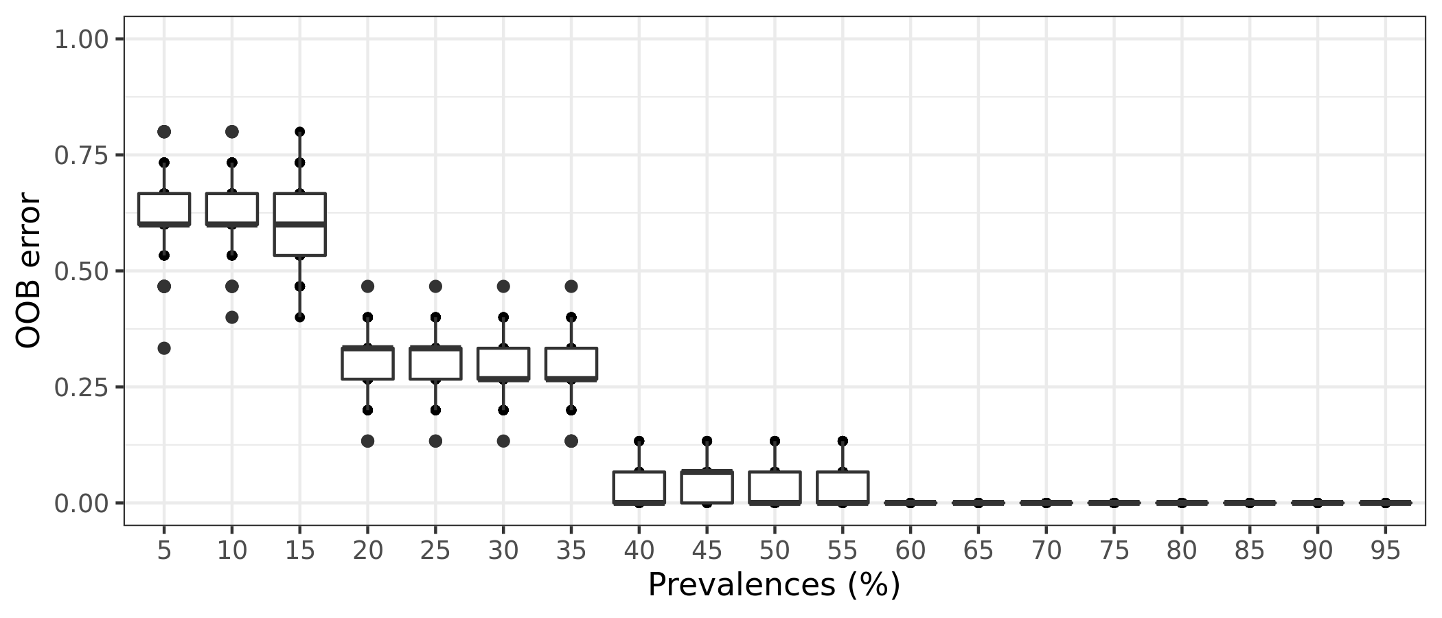
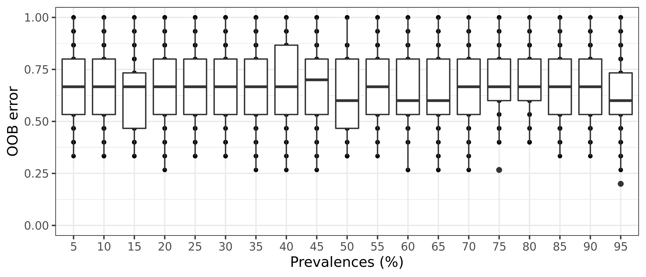
Estimate Error in Prediction
Using the function pime.error.prediction we can estimate the error in prediction. For each prevalence interval, this function randomizes the samples labels into arbitrary groupings using n random permutations, defined by the bootstrap value. For each, randomized and prevalence filtered, data set the OOB error rate is calculated to estimate whether the original differences in groups of samples occur by chance. Results are in a list containing a table and a box plot summarizing the results.
(16S rRNA) Table 8 | Results of 100 random permutations for each prevalence interval based on a function that randomizes the samples labels into arbitrary groupings. using n random permutations. For each randomized and prevalence filtered data set, the OOB error rate is calculated to estimate whether the original differences in groups of samples occur by chance.
It is also possible to estimate the variation of OOB error for each prevalence interval filtering. This is done by running the random forests classification for n times, determined by the bootstrap value. The function will return a box plot figure and a table for each classification error.
298 OTUs were removed because they are no longer
present in any sample after random subsampling
phyloseq-class experiment-level object
otu_table()   OTU Table:         [ 3057 taxa and 13 samples ]
sample_data() Sample Data:       [ 13 samples by 6 sample variables ]
tax_table()   Taxonomy Table:    [ 3057 taxa by 8 taxonomic ranks ]
The first step in PIME is to define if the microbial community presents a high relative abundance of taxa with low prevalence, which is considered as noise in PIME analysis. This is calculated by random forests analysis and is the baseline noise detection.
$`0`
phyloseq-class experiment-level object
otu_table()   OTU Table:         [ 1932 taxa and 5 samples ]
sample_data() Sample Data:       [ 5 samples by 6 sample variables ]
tax_table()   Taxonomy Table:    [ 1932 taxa by 8 taxonomic ranks ]

$`3`
phyloseq-class experiment-level object
otu_table()   OTU Table:         [ 1682 taxa and 4 samples ]
sample_data() Sample Data:       [ 4 samples by 6 sample variables ]
tax_table()   Taxonomy Table:    [ 1682 taxa by 8 taxonomic ranks ]

$`8`
phyloseq-class experiment-level object
otu_table()   OTU Table:         [ 1306 taxa and 4 samples ]
sample_data() Sample Data:       [ 4 samples by 6 sample variables ]
tax_table()   Taxonomy Table:    [ 1306 taxa by 8 taxonomic ranks ]
Calculate Prevalence Intervals
Using the output of pime.split.by.variable, we calculate the prevalence intervals with the function pime.prevalence. This function estimates the highest prevalence possible (no empty ASV table), calculates prevalence for taxa, starting at 5 maximum prevalence possible (no empty ASV table or dropping samples). After prevalence calculation, each prevalence interval are merged.
$`5`
phyloseq-class experiment-level object
otu_table()   OTU Table:         [ 3057 taxa and 13 samples ]
sample_data() Sample Data:       [ 13 samples by 6 sample variables ]
tax_table()   Taxonomy Table:    [ 3057 taxa by 8 taxonomic ranks ]

$`10`
phyloseq-class experiment-level object
otu_table()   OTU Table:         [ 3057 taxa and 13 samples ]
sample_data() Sample Data:       [ 13 samples by 6 sample variables ]
tax_table()   Taxonomy Table:    [ 3057 taxa by 8 taxonomic ranks ]

$`15`
phyloseq-class experiment-level object
otu_table()   OTU Table:         [ 3057 taxa and 13 samples ]
sample_data() Sample Data:       [ 13 samples by 6 sample variables ]
tax_table()   Taxonomy Table:    [ 3057 taxa by 8 taxonomic ranks ]

$`20`
phyloseq-class experiment-level object
otu_table()   OTU Table:         [ 2421 taxa and 13 samples ]
sample_data() Sample Data:       [ 13 samples by 6 sample variables ]
tax_table()   Taxonomy Table:    [ 2421 taxa by 8 taxonomic ranks ]

$`25`
phyloseq-class experiment-level object
otu_table()   OTU Table:         [ 1152 taxa and 13 samples ]
sample_data() Sample Data:       [ 13 samples by 6 sample variables ]
tax_table()   Taxonomy Table:    [ 1152 taxa by 8 taxonomic ranks ]

$`30`
phyloseq-class experiment-level object
otu_table()   OTU Table:         [ 1152 taxa and 13 samples ]
sample_data() Sample Data:       [ 13 samples by 6 sample variables ]
tax_table()   Taxonomy Table:    [ 1152 taxa by 8 taxonomic ranks ]

$`35`
phyloseq-class experiment-level object
otu_table()   OTU Table:         [ 1152 taxa and 13 samples ]
sample_data() Sample Data:       [ 13 samples by 6 sample variables ]
tax_table()   Taxonomy Table:    [ 1152 taxa by 8 taxonomic ranks ]

$`40`
phyloseq-class experiment-level object
otu_table()   OTU Table:         [ 873 taxa and 13 samples ]
sample_data() Sample Data:       [ 13 samples by 6 sample variables ]
tax_table()   Taxonomy Table:    [ 873 taxa by 8 taxonomic ranks ]

$`45`
phyloseq-class experiment-level object
otu_table()   OTU Table:         [ 873 taxa and 13 samples ]
sample_data() Sample Data:       [ 13 samples by 6 sample variables ]
tax_table()   Taxonomy Table:    [ 873 taxa by 8 taxonomic ranks ]

$`50`
phyloseq-class experiment-level object
otu_table()   OTU Table:         [ 474 taxa and 13 samples ]
sample_data() Sample Data:       [ 13 samples by 6 sample variables ]
tax_table()   Taxonomy Table:    [ 474 taxa by 8 taxonomic ranks ]

$`55`
phyloseq-class experiment-level object
otu_table()   OTU Table:         [ 474 taxa and 13 samples ]
sample_data() Sample Data:       [ 13 samples by 6 sample variables ]
tax_table()   Taxonomy Table:    [ 474 taxa by 8 taxonomic ranks ]

$`60`
phyloseq-class experiment-level object
otu_table()   OTU Table:         [ 336 taxa and 13 samples ]
sample_data() Sample Data:       [ 13 samples by 6 sample variables ]
tax_table()   Taxonomy Table:    [ 336 taxa by 8 taxonomic ranks ]

$`65`
phyloseq-class experiment-level object
otu_table()   OTU Table:         [ 336 taxa and 13 samples ]
sample_data() Sample Data:       [ 13 samples by 6 sample variables ]
tax_table()   Taxonomy Table:    [ 336 taxa by 8 taxonomic ranks ]

$`70`
phyloseq-class experiment-level object
otu_table()   OTU Table:         [ 336 taxa and 13 samples ]
sample_data() Sample Data:       [ 13 samples by 6 sample variables ]
tax_table()   Taxonomy Table:    [ 336 taxa by 8 taxonomic ranks ]

$`75`
phyloseq-class experiment-level object
otu_table()   OTU Table:         [ 171 taxa and 13 samples ]
sample_data() Sample Data:       [ 13 samples by 6 sample variables ]
tax_table()   Taxonomy Table:    [ 171 taxa by 8 taxonomic ranks ]

$`80`
phyloseq-class experiment-level object
otu_table()   OTU Table:         [ 114 taxa and 13 samples ]
sample_data() Sample Data:       [ 13 samples by 6 sample variables ]
tax_table()   Taxonomy Table:    [ 114 taxa by 8 taxonomic ranks ]

$`85`
phyloseq-class experiment-level object
otu_table()   OTU Table:         [ 114 taxa and 13 samples ]
sample_data() Sample Data:       [ 13 samples by 6 sample variables ]
tax_table()   Taxonomy Table:    [ 114 taxa by 8 taxonomic ranks ]

$`90`
phyloseq-class experiment-level object
otu_table()   OTU Table:         [ 114 taxa and 13 samples ]
sample_data() Sample Data:       [ 13 samples by 6 sample variables ]
tax_table()   Taxonomy Table:    [ 114 taxa by 8 taxonomic ranks ]

$`95`
phyloseq-class experiment-level object
otu_table()   OTU Table:         [ 114 taxa and 13 samples ]
sample_data() Sample Data:       [ 13 samples by 6 sample variables ]
tax_table()   Taxonomy Table:    [ 114 taxa by 8 taxonomic ranks ]
Calculate Best Prevalence
Finally, we use the function pime.best.prevalence to calculate the best prevalence. The function uses randomForest to build random forests trees for samples classification and variable importance computation. It performs classifications for each prevalence interval returned by pime.prevalence. Variable importance is calculated, returning the Mean Decrease Accuracy (MDA), Mean Decrease Impurity (MDI), overall and by sample group, and taxonomy for each ASV. PIME keeps the top 30 variables with highest MDA each prevalence level.
phyloseq-class experiment-level object
otu_table()   OTU Table:         [ 474 taxa and 13 samples ]
sample_data() Sample Data:       [ 13 samples by 6 sample variables ]
tax_table()   Taxonomy Table:    [ 474 taxa by 8 taxonomic ranks ]
(ITS) Table 5 | Summary of PERfect filtering using the defualt order and filtering p-values < 0.10.
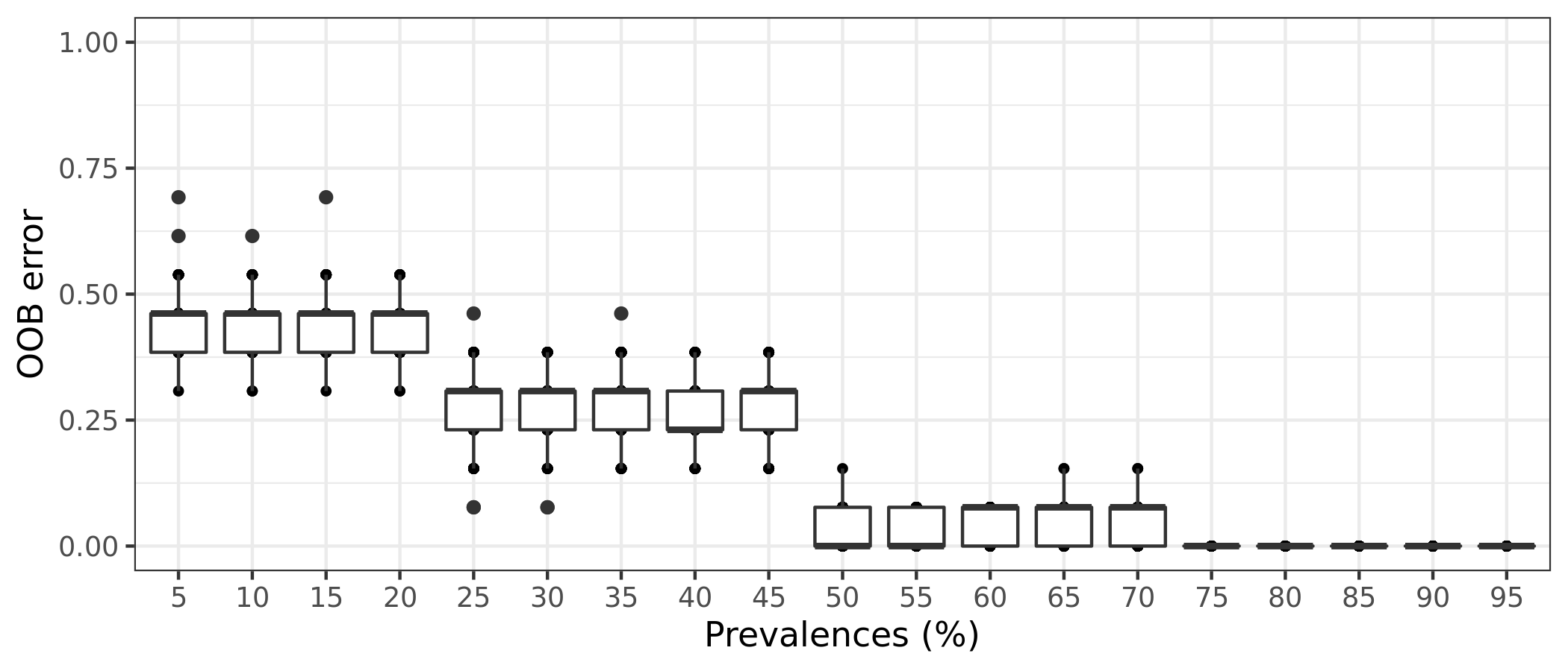
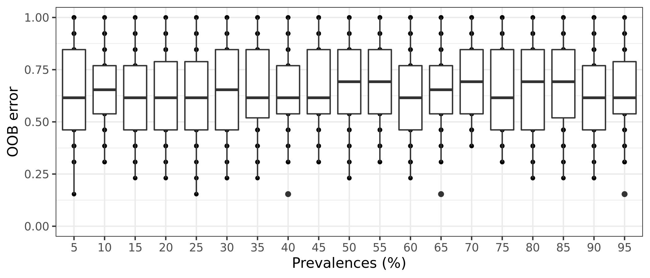
Estimate Error in Prediction
Using the function pime.error.prediction we can estimate the error in prediction. For each prevalence interval, this function randomizes the samples labels into arbitrary groupings using n random permutations, defined by the bootstrap value. For each, randomized and prevalence filtered, data set the OOB error rate is calculated to estimate whether the original differences in groups of samples occur by chance. Results are in a list containing a table and a box plot summarizing the results.
(ITS) Table 8 | Results of 100 random permutations for each prevalence interval based on a function that randomizes the samples labels into arbitrary groupings. using n random permutations. For each randomized and prevalence filtered data set, the OOB error rate is calculated to estimate whether the original differences in groups of samples occur by chance.
It is also possible to estimate the variation of OOB error for each prevalence interval filtering. This is done by running the random forests classification for n times, determined by the bootstrap value. The function will return a box plot figure and a table for each classification error.
The source code for this page can be accessed on GitHub by clicking this link.
Data Availability
Data generated in this workflow and the Rdata file need to run the workflow can be accessed on figshare at 10.25573/data.14701440.
Last updated on
[1] "2025-08-23 13:27:42 PDT"
References
Roesch, Luiz Fernando W, Priscila T Dobbler, Victor S Pylro, Bryan Kolaczkowski, Jennifer C Drew, and Eric W Triplett. 2020. “PIME: A Package for Discovery of Novel Differences Among Microbial Communities.”Molecular Ecology Resources 20 (2): 415–28. https://doi.org/10.1111/1755-0998.13116.
Smirnova, Ekaterina, Snehalata Huzurbazar, and Farhad Jafari. 2019. “PERFect: PERmutation Filtering Test for Microbiome Data.”Biostatistics 20 (4): 615–31. https://doi.org/10.1093/biostatistics/kxy020.
Source Code
---title: "3. Filtering"description: | Reproducible workflow for Arbitrary, PERfect, & PIME filtering of community data.format: html: toc: true toc-depth: 3---```{r}#| message: false#| results: hide#| code-fold: true#| code-summary: "Click here for setup information"remove(list =ls())knitr::opts_chunk$set(echo =TRUE, eval =FALSE)set.seed(119)#library(conflicted)#pacman::p_depends(PERFect, local = TRUE) #pacman::p_depends_reverse(PERFect, local = TRUE) library(phyloseq); packageVersion("phyloseq")library(Biostrings); packageVersion("Biostrings")pacman::p_load(tidyverse, patchwork, agricolae, labdsv, naniar, PERFect, pime, ape, gdata, pairwiseAdonis, microbiome, seqRFLP, microbiomeMarker, reactable, downloadthis, captioner, jamba, install =FALSE, update =FALSE)library(ggstatsplot)library(ggside)options(scipen=999)knitr::opts_current$get(c("cache","cache.path","cache.rebuild","dependson","autodep"))source(file.path("assets", "functions.R"))``````{r}#| include: false#| eval: true## Load to build pageload("page_build/filtering_wf.rdata")ssu18_ps_work <-readRDS("files/data-prep/rdata/ssu18_ps_work.rds")its18_ps_work <-readRDS("files/data-prep/rdata/its18_ps_work.rds")``````{r}#| include: false#| eval: true#| results: hide# Create the caption(s) with captionercaption_tab_ssu <-captioner(prefix ="(16S rRNA) Table", suffix =" |", style ="b")caption_fig_ssu <-captioner(prefix ="(16S rRNA) Figure", suffix =" |", style ="b")caption_tab_its <-captioner(prefix ="(ITS) Table", suffix =" |", style ="b")caption_fig_its <-captioner(prefix ="(ITS) Figure", suffix =" |", style ="b")# Create a function for referring to the tables in textref <-function(x) str_extract(x, "[^|]*") %>%trimws(which ="right", whitespace ="[ ]")```</details>```{r}#| echo: false#| eval: truesource("assets/captions/captions_filtering.R")```In [Part A](#a.-arbitrary-filtering), we apply arbitrary filtering to the 16S rRNA and ITS data sets. In [Part B](#b.-perfect-filtering) we use PERFect [(PERmutation Filtering test for microbiome data)](https://github.com/katiasmirn/PERFect)[@smirnova2019perfect] to filter the data sets. And in [Part C](#c.-pime-filtering) of this workflow, we use PIME [(Prevalence Interval for Microbiome Evaluation)](https://github.com/microEcology/pime)[@roesch2020pime] to filter the FULL 16S rRNA and ITS data sets. ## Workflow InputFiles needed to run this workflow can be downloaded from figshare. <iframe src="https://widgets.figshare.com/articles/14690739/embed?show_title=1" width="100%" height="301" allowfullscreen frameborder="0"></iframe># Filtering ResultsWe begin by summarizing the results of each filtering method on the 16S and ITS data sets. Below you can find the complete workflow for each filtering method.## 16S rRNA<small>`r caption_tab_ssu("ssu_all_filt_summary")`</small>```{r}#| echo: falsessu18_filtering_results <- dplyr::left_join(ssu18_sum_arbitrary, ssu18_sum_perfect, by =c("Metric", "Full data")) %>% dplyr::left_join(., ssu18_sum_pime, by =c("Metric", "Full data")) %>% dplyr::rename("Arbitrary"=3, "PERfect"=4, "PIME"=5)``````{r}#| echo: false#| eval: trueseq_table <- ssu18_filtering_resultswrite.table(seq_table, "files/filtering/tables/ssu_all_filt_summary.txt", row.names =FALSE, sep ="\t", quote =FALSE)``````{r}#| echo: false#| eval: truereactable(seq_table,defaultColDef =colDef(header =function(value) gsub("_", " ", value, fixed =TRUE),cell =function(value) format(value, nsmall =0),align ="center", filterable =FALSE, sortable =TRUE, resizable =TRUE,footerStyle =list(fontWeight ="bold"), minWidth =100 ), columns =list(Metric =colDef(name ="Metric", sticky ="left", style =list(borderRight ="1px solid #eee"),headerStyle =list(borderRight ="1px solid #eee"), align ="left",minWidth =200) ), searchable =FALSE, defaultPageSize =10, showPagination =FALSE,pageSizeOptions =c(5, 10, nrow(seq_table)), showPageSizeOptions =TRUE, highlight =TRUE, bordered =TRUE, striped =TRUE, compact =TRUE, wrap =FALSE, showSortable =FALSE, fullWidth =TRUE,theme =reactableTheme(style =list(fontSize ="0.8em")))rm(seq_table)```{{< downloadthis files/filtering/tables/ssu_all_filt_summary.txt dname="ssu_all_filt_summary" label="Download table as text file" icon="table" type="primary" >}}```{r}#| echo: falsetmp_read_count <-data.frame(sample_sums(ssu18_ps_work)) %>% tibble::rownames_to_column("SamName")tmp_asv_count <-estimate_richness(ssu18_ps_work, split =TRUE, measures ="Observed") %>% tibble::rownames_to_column("SamName")tmp_samp_data <-data.frame(sample_data(ssu18_ps_work))tmp_samp_data <- tmp_samp_data[order(tmp_samp_data$PLOT, tmp_samp_data$TEMP),]tmp_join <- dplyr::left_join(tmp_samp_data, tmp_read_count, by ="SamName") %>% dplyr::left_join(., tmp_asv_count, by ="SamName") %>% dplyr::rename("Sample_ID"=1) %>% dplyr::rename("total_reads"=7) %>% dplyr::rename("total_asvs"=8)tmp_join[, 3] <-NULLssu_work_samp_summary <- tmp_joinrm(list =ls(pattern ="tmp_"))``````{r}#| echo: falsessu18_filtering_results <- dplyr::left_join(ssu18_sum_arbitrary, ssu18_sum_perfect, by =c("Metric", "Full data")) %>% dplyr::left_join(., ssu18_sum_pime, by =c("Metric", "Full data")) %>% dplyr::rename("Arbitrary"=3, "PERfect"=4, "PIME"=5)``````{r}#| echo: falsessu_all_filt_samp_summary <- dplyr::left_join(ssu_work_samp_summary, ssu_filt_samp_summary, by =c("Sample_ID", "PLOT", "TREAT", "TEMP", "PAIR")) %>% dplyr::left_join(., ssu_perfect_samp_summary, by =c("Sample_ID", "PLOT", "TREAT", "TEMP", "PAIR")) %>% dplyr::left_join(., ssu_pime_samp_summary, by =c("Sample_ID", "PLOT", "TREAT", "TEMP", "PAIR")) %>% dplyr::relocate(c("total_reads.x", "total_reads.y", "total_reads.x.x", "total_reads.y.y"), .after ="PAIR")ssu_all_filt_samp_summary[,2:5] <-NULL```<small>`r caption_tab_ssu("ssu_all_filt_samp_summary")`</small>```{r}#| echo: false#| eval: trueseq_table <- ssu_all_filt_samp_summarywrite.table(seq_table, "files/filtering/tables/ssu_all_filt_samp_summary.txt", row.names =FALSE, sep ="\t", quote =FALSE)``````{r}#| echo: false#| eval: truereactable(seq_table,columns =list(Sample_ID =colDef(name ="Sample_ID", sticky ="left", style =list(borderRight ="5px solid #eee"),headerStyle =list(borderRight ="5px solid #eee"), align ="left",minWidth =150),total_reads.x =colDef(name ="FULL"),total_reads.y =colDef(name ="Arbitrary"),total_reads.x.x =colDef(name ="PERfect"),total_reads.y.y =colDef(name ="PIME", style =list(borderRight ="5px solid #eee"),headerStyle =list(borderRight ="5px solid #eee")),total_asvs.x =colDef(name ="FULL"),total_asvs.y =colDef(name ="Arbitrary"),total_asvs.x.x =colDef(name ="PERfect"),total_asvs.y.y =colDef(name ="PIME") ),columnGroups =list(colGroup(name ="Total Reads", columns =c("total_reads.x", "total_reads.y", "total_reads.x.x", "total_reads.y.y"),headerStyle =list(borderRight ="5px solid #eee", fontSize ="1.5em")),colGroup(name ="Total ASVs", columns =c("total_asvs.x", "total_asvs.y", "total_asvs.x.x", "total_asvs.y.y"),headerStyle =list(fontSize ="1.5em")) ),defaultColDef =colDef(header =function(value) gsub("_", " ", value, fixed =TRUE),cell =function(value) format(value, nsmall =0),align ="center", filterable =TRUE, sortable =TRUE, resizable =TRUE,footerStyle =list(fontWeight ="bold"), minWidth =100 ), searchable =TRUE, defaultPageSize =5, showPagination =TRUE,pageSizeOptions =c(5, 10, nrow(seq_table)), showPageSizeOptions =TRUE, highlight =TRUE, bordered =TRUE, striped =TRUE, compact =TRUE, wrap =FALSE, showSortable =TRUE, fullWidth =TRUE,theme =reactableTheme(style =list(fontSize ="0.8em")))rm(seq_table)```{{< downloadthis files/filtering/tables/ssu_all_filt_samp_summary.txt dname="ssu_all_filt_samp_summary" label="Download table as text file" icon="table" type="primary" >}}## ITS<small>`r caption_tab_its("its_all_filt_summary")`</small>```{r}#| echo: falseits18_filtering_results <- dplyr::left_join(its18_sum_arbitrary, its18_sum_perfect, by =c("Metric", "Full data")) %>% dplyr::left_join(., its18_sum_pime, by =c("Metric", "Full data")) %>% dplyr::rename("Arbitrary"=3, "PERfect"=4, "PIME"=5)``````{r}#| echo: false#| eval: trueseq_table <- its18_filtering_resultswrite.table(seq_table, "files/filtering/tables/its_all_filt_summary.txt", row.names =FALSE, sep ="\t", quote =FALSE)``````{r}#| echo: false#| eval: truereactable(seq_table,defaultColDef =colDef(header =function(value) gsub("_", " ", value, fixed =TRUE),cell =function(value) format(value, nsmall =0),align ="center", filterable =FALSE, sortable =TRUE, resizable =TRUE,footerStyle =list(fontWeight ="bold"), minWidth =100 ), columns =list(Metric =colDef(name ="Metric", sticky ="left", style =list(borderRight ="1px solid #eee"),headerStyle =list(borderRight ="1px solid #eee"), align ="left",minWidth =200) ), searchable =FALSE, defaultPageSize =10, showPagination =FALSE,pageSizeOptions =c(5, 10, nrow(seq_table)), showPageSizeOptions =TRUE, highlight =TRUE, bordered =TRUE, striped =TRUE, compact =TRUE, wrap =FALSE, showSortable =FALSE, fullWidth =TRUE,theme =reactableTheme(style =list(fontSize ="0.8em")))rm(seq_table)```{{< downloadthis files/filtering/tables/its_all_filt_summary.txt dname="its_all_filt_summary" label="Download table as text file" icon="table" type="primary" >}}```{r}#| echo: falsetmp_read_count <-data.frame(sample_sums(its18_ps_work)) %>% tibble::rownames_to_column("SamName")tmp_asv_count <-estimate_richness(its18_ps_work, split =TRUE, measures ="Observed") %>% tibble::rownames_to_column("SamName")tmp_samp_data <-data.frame(sample_data(its18_ps_work))tmp_samp_data <- tmp_samp_data[order(tmp_samp_data$PLOT, tmp_samp_data$TEMP),]tmp_join <- dplyr::left_join(tmp_samp_data, tmp_read_count, by ="SamName") %>% dplyr::left_join(., tmp_asv_count, by ="SamName") %>% dplyr::rename("Sample_ID"=1) %>% dplyr::rename("total_reads"=7) %>% dplyr::rename("total_asvs"=8)tmp_join[, 3] <-NULLits_work_samp_summary <- tmp_joinrm(list =ls(pattern ="tmp_"))``````{r}#| echo: falseits18_filtering_results <- dplyr::left_join(its18_sum_arbitrary, its18_sum_perfect, by =c("Metric", "Full data")) %>% dplyr::left_join(., its18_sum_pime, by =c("Metric", "Full data")) %>% dplyr::rename("Arbitrary"=3, "PERfect"=4, "PIME"=5)``````{r}#| echo: falseits_all_filt_samp_summary <- dplyr::left_join(its_work_samp_summary, its_filt_samp_summary, by =c("Sample_ID", "PLOT", "TREAT", "TEMP", "PAIR")) %>% dplyr::left_join(., its_perfect_samp_summary, by =c("Sample_ID", "PLOT", "TREAT", "TEMP", "PAIR")) %>% dplyr::left_join(., its_pime_samp_summary, by =c("Sample_ID", "PLOT", "TREAT", "TEMP", "PAIR")) %>% dplyr::relocate(c("total_reads.x", "total_reads.y", "total_reads.x.x", "total_reads.y.y"), .after ="PAIR")its_all_filt_samp_summary[,2:5] <-NULL```<small>`r caption_tab_its("its_all_filt_samp_summary")`</small>```{r}#| echo: false#| eval: trueseq_table <- its_all_filt_samp_summarywrite.table(seq_table, "files/filtering/tables/its_all_filt_samp_summary.txt", row.names =FALSE, sep ="\t", quote =FALSE)``````{r}#| echo: false#| eval: truereactable(seq_table,columns =list(Sample_ID =colDef(name ="Sample_ID", sticky ="left", style =list(borderRight ="5px solid #eee"),headerStyle =list(borderRight ="5px solid #eee"), align ="left",minWidth =150),total_reads.x =colDef(name ="FULL"),total_reads.y =colDef(name ="Arbitrary"),total_reads.x.x =colDef(name ="PERfect"),total_reads.y.y =colDef(name ="PIME", style =list(borderRight ="5px solid #eee"),headerStyle =list(borderRight ="5px solid #eee")),total_asvs.x =colDef(name ="FULL"),total_asvs.y =colDef(name ="Arbitrary"),total_asvs.x.x =colDef(name ="PERfect"),total_asvs.y.y =colDef(name ="PIME") ),columnGroups =list(colGroup(name ="Total Reads", columns =c("total_reads.x", "total_reads.y", "total_reads.x.x", "total_reads.y.y"),headerStyle =list(borderRight ="5px solid #eee", fontSize ="1.5em")),colGroup(name ="Total ASVs", columns =c("total_asvs.x", "total_asvs.y", "total_asvs.x.x", "total_asvs.y.y"),headerStyle =list(fontSize ="1.5em")) ),defaultColDef =colDef(header =function(value) gsub("_", " ", value, fixed =TRUE),cell =function(value) format(value, nsmall =0),align ="center", filterable =TRUE, sortable =TRUE, resizable =TRUE,footerStyle =list(fontWeight ="bold"), minWidth =100 ), searchable =TRUE, defaultPageSize =5, showPagination =TRUE,pageSizeOptions =c(5, 10, nrow(seq_table)), showPageSizeOptions =TRUE, highlight =TRUE, bordered =TRUE, striped =TRUE, compact =TRUE, wrap =FALSE, showSortable =TRUE, fullWidth =TRUE,theme =reactableTheme(style =list(fontSize ="0.8em")))rm(seq_table)```{{< downloadthis files/filtering/tables/its_all_filt_samp_summary.txt dname="its_all_filt_samp_summary" label="Download table as text file" icon="table" type="primary" >}}# A. Arbitrary FilteringFor low-count arbitrary filtering, we set the minimum read count to `5` and the prevalence to 20%. Then we apply another filter to remove ASVs with a low variance (`0.2`).```{r}#| include: false## Initial Load for ARBITRARY ANALYSIS #1set.seed(119)ssu18_ps_work <-readRDS("files/data-prep/rdata/ssu18_ps_work.rds")its18_ps_work <-readRDS("files/data-prep/rdata/its18_ps_work.rds")```## 16S rRNA```{r}#| code-fold: truetmp_low_count <- phyloseq::genefilter_sample( ssu18_ps_work, filterfun_sample(function(x) x >=5), A =0.2*nsamples(ssu18_ps_work))tmp_low_count <- phyloseq::prune_taxa(tmp_low_count, ssu18_ps_work)tmp_low_var <- phyloseq::filter_taxa(tmp_low_count, function(x) var(x) >0.2, prune =TRUE)ssu18_ps_filt <- tmp_low_varssu18_ps_filt@phy_tree <-NULLtmp_tree <-rtree(ntaxa(ssu18_ps_filt), rooted =TRUE,tip.label =taxa_names(ssu18_ps_filt))ssu18_ps_filt <-merge_phyloseq(ssu18_ps_filt, sample_data, tmp_tree)rm(list =ls(pattern ="tmp_"))ssu18_ps_filt```Here is the filtered 16S rRNA phyloseq object. ```{r}#| echo: false#| eval: truessu18_ps_filt``````{r}#| echo: false## This code is gross. I spent hours trying to find a better## solution but failed :(rm(list =ls(pattern ="tmp_"))tmp_samples <-c("ssu18_ps_work", "ssu18_ps_filt")tmp_objects <-c("Total number of reads", "Min. number of reads", "Max. number of reads", "Average number of reads", "Median number of reads", "Total ASVs", "Min. number of ASVs", "Max. number of ASVs", "Average number of ASVs", "Median number of ASVs")tmp_total_reads <-c()for (i in tmp_samples) { tmp_get <-sum(readcount(get(i))) tmp_total_reads <-c(append(tmp_total_reads, tmp_get))}tmp_min_read <-c()for (i in tmp_samples) { tmp_get <-min(readcount(get(i))) tmp_min_read <-c(append(tmp_min_read, tmp_get))}tmp_max_read <-c()for (i in tmp_samples) { tmp_get <-max(readcount(get(i))) tmp_max_read <-c(append(tmp_max_read, tmp_get))}tmp_mean_reads <-c()for (i in tmp_samples) { tmp_get <-round(mean(readcount(get(i))), digits =0) tmp_mean_reads <-c(append(tmp_mean_reads, tmp_get))}tmp_median_reads <-c()for (i in tmp_samples) { tmp_get <-median(readcount(get(i))) tmp_median_reads <-c(append(tmp_median_reads, tmp_get))}tmp_total_asvs <-c()for (i in tmp_samples) { tmp_get <-ntaxa(get(i)) tmp_total_asvs <-c(append(tmp_total_asvs, tmp_get))}tmp_min_asvs <-c()for (i in tmp_samples) { tmp_get <-min(richness(get(i), index ="observed")) tmp_min_asvs <-c(append(tmp_min_asvs, tmp_get))}tmp_max_asvs <-c()for (i in tmp_samples) { tmp_get <-max(richness(get(i), index ="observed")) tmp_max_asvs <-c(append(tmp_max_asvs, tmp_get))}tmp_mean_asvs <-c()for (i in tmp_samples) { tmp_get <-round(mean(richness(get(i), index ="observed")$observed), digits =0) tmp_mean_asvs <-c(append(tmp_mean_asvs, tmp_get))}tmp_med_asvs <-c()for (i in tmp_samples) { tmp_get <-median(richness(get(i), index ="observed")$observed) tmp_med_asvs <-c(append(tmp_med_asvs, tmp_get))}tmp_bind <-data.frame(do.call("rbind", list( tmp_total_reads, tmp_min_read, tmp_max_read, tmp_mean_reads, tmp_median_reads, tmp_total_asvs, tmp_min_asvs, tmp_max_asvs, tmp_mean_asvs, tmp_med_asvs)))ssu18_sum_arbitrary <- dplyr::bind_cols(tmp_objects, tmp_bind) %>% dplyr::rename("Metric"=1, "Full data"=2, "Arbitrary filter"=3)rm(list =ls(pattern ="tmp_"))```<small>`r caption_tab_ssu("ssu_arbitrary_filt_summary")`</small>```{r}#| echo: false#| eval: trueseq_table <- ssu18_sum_arbitrarywrite.table(seq_table, "files/filtering/tables/ssu_arbitrary_filt_summary.txt", row.names =FALSE, sep ="\t", quote =FALSE)``````{r}#| echo: false#| eval: truereactable(seq_table,defaultColDef =colDef(header =function(value) gsub("_", " ", value, fixed =TRUE),cell =function(value) format(value, nsmall =0),align ="center", filterable =FALSE, sortable =TRUE, resizable =TRUE,footerStyle =list(fontWeight ="bold"), minWidth =150 ), columns =list(Metric =colDef(name ="Metric", sticky ="left", style =list(borderRight ="1px solid #eee"),headerStyle =list(borderRight ="1px solid #eee"), align ="left",minWidth =200) ), searchable =FALSE, defaultPageSize =10, showPagination =FALSE,pageSizeOptions =c(5, 10, nrow(seq_table)), showPageSizeOptions =TRUE, highlight =TRUE, bordered =TRUE, striped =TRUE, compact =TRUE, wrap =FALSE, showSortable =FALSE, fullWidth =TRUE,theme =reactableTheme(style =list(fontSize ="0.8em")))rm(seq_table)```{{< downloadthis files/filtering/tables/ssu_arbitrary_filt_summary.txt dname="ssu_arbitrary_filt_summary" label="Download table as text file" icon="table" type="primary" >}}We can look at how filtering affected total reads and ASVs for each sample.```{r}#| echo: falsetmp_read_count <-data.frame(sample_sums(ssu18_ps_filt)) %>% tibble::rownames_to_column("SamName")tmp_asv_count <-estimate_richness(ssu18_ps_filt, split =TRUE, measures ="Observed") %>% tibble::rownames_to_column("SamName")tmp_samp_data <-data.frame(sample_data(ssu18_ps_filt))tmp_samp_data <- tmp_samp_data[order(tmp_samp_data$PLOT, tmp_samp_data$TEMP),]tmp_join <- dplyr::left_join(tmp_samp_data, tmp_read_count, by ="SamName") %>% dplyr::left_join(., tmp_asv_count, by ="SamName") %>% dplyr::rename("Sample_ID"=1) %>% dplyr::rename("total_reads"=7) %>% dplyr::rename("total_asvs"=8)tmp_join[, 3] <-NULLssu_filt_samp_summary <- tmp_joinrm(list =ls(pattern ="tmp_"))```<small>`r caption_tab_ssu("ssu_filt_samp_summary")`</small>```{r}#| echo: false#| eval: trueseq_table <- ssu_filt_samp_summarywrite.table(seq_table, "files/filtering/tables/ssu_filt_samp_summary.txt", row.names =FALSE, sep ="\t", quote =FALSE)``````{r}#| echo: false#| eval: truereactable(seq_table,defaultColDef =colDef(header =function(value) gsub("_", " ", value, fixed =TRUE),cell =function(value) format(value, nsmall =0),align ="center", filterable =TRUE, sortable =TRUE, resizable =TRUE,footerStyle =list(fontWeight ="bold"), minWidth =100 ), columns =list(Sample_ID =colDef(name ="Sample_ID", sticky ="left", style =list(borderRight ="1px solid #eee"),headerStyle =list(borderRight ="1px solid #eee"), align ="left",minWidth =150) ), searchable =TRUE, defaultPageSize =5, showPagination =TRUE,pageSizeOptions =c(5, 10, nrow(seq_table)), showPageSizeOptions =TRUE, highlight =TRUE, bordered =TRUE, striped =TRUE, compact =TRUE, wrap =FALSE, showSortable =TRUE, fullWidth =FALSE,theme =reactableTheme(style =list(fontSize ="0.8em")))rm(seq_table)```{{< downloadthis files/filtering/tables/ssu_filt_samp_summary.txt dname="ssu_filt_samp_summary" label="Download table as text file" icon="table" type="primary" >}}## ITS```{r}#| code-fold: truetmp_low_count <- phyloseq::genefilter_sample( its18_ps_work, filterfun_sample(function(x) x >=5), A =0.2*nsamples(its18_ps_work))tmp_low_count <- phyloseq::prune_taxa(tmp_low_count, its18_ps_work)tmp_low_var <- phyloseq::filter_taxa(tmp_low_count, function(x) var(x) >0.2, prune =TRUE)its18_ps_filt <- tmp_low_varrm(list =ls(pattern ="tmp_"))its18_ps_filt```And the filtered ITS phyloseq object. ```{r}#| echo: false#| eval: trueits18_ps_filt``````{r}#| echo: false## This code is gross. I spent hours trying to find a better## solution but failed :(rm(list =ls(pattern ="tmp_"))tmp_samples <-c("its18_ps_work", "its18_ps_filt")tmp_objects <-c("Total number of reads", "Min. number of reads", "Max. number of reads", "Average number of reads", "Median number of reads", "Total ASVs", "Min. number of ASVs", "Max. number of ASVs", "Average number of ASVs", "Median number of ASVs")tmp_total_reads <-c()for (i in tmp_samples) { tmp_get <-sum(readcount(get(i))) tmp_total_reads <-c(append(tmp_total_reads, tmp_get))}tmp_min_read <-c()for (i in tmp_samples) { tmp_get <-min(readcount(get(i))) tmp_min_read <-c(append(tmp_min_read, tmp_get))}tmp_max_read <-c()for (i in tmp_samples) { tmp_get <-max(readcount(get(i))) tmp_max_read <-c(append(tmp_max_read, tmp_get))}tmp_mean_reads <-c()for (i in tmp_samples) { tmp_get <-round(mean(readcount(get(i))), digits =0) tmp_mean_reads <-c(append(tmp_mean_reads, tmp_get))}tmp_median_reads <-c()for (i in tmp_samples) { tmp_get <-median(readcount(get(i))) tmp_median_reads <-c(append(tmp_median_reads, tmp_get))}tmp_total_asvs <-c()for (i in tmp_samples) { tmp_get <-ntaxa(get(i)) tmp_total_asvs <-c(append(tmp_total_asvs, tmp_get))}tmp_min_asvs <-c()for (i in tmp_samples) { tmp_get <-min(richness(get(i), index ="observed")) tmp_min_asvs <-c(append(tmp_min_asvs, tmp_get))}tmp_max_asvs <-c()for (i in tmp_samples) { tmp_get <-max(richness(get(i), index ="observed")) tmp_max_asvs <-c(append(tmp_max_asvs, tmp_get))}tmp_mean_asvs <-c()for (i in tmp_samples) { tmp_get <-round(mean(richness(get(i), index ="observed")$observed), digits =0) tmp_mean_asvs <-c(append(tmp_mean_asvs, tmp_get))}tmp_med_asvs <-c()for (i in tmp_samples) { tmp_get <-median(richness(get(i), index ="observed")$observed) tmp_med_asvs <-c(append(tmp_med_asvs, tmp_get))}tmp_bind <-data.frame(do.call("rbind", list( tmp_total_reads, tmp_min_read, tmp_max_read, tmp_mean_reads, tmp_median_reads, tmp_total_asvs, tmp_min_asvs, tmp_max_asvs, tmp_mean_asvs, tmp_med_asvs)))its18_sum_arbitrary <- dplyr::bind_cols(tmp_objects, tmp_bind) %>% dplyr::rename("Metric"=1, "Full data"=2, "Arbitrary filter"=3)rm(list =ls(pattern ="tmp_"))```<small>`r caption_tab_its("its_arbitrary_filt_summary")`</small>```{r}#| echo: false#| eval: trueseq_table <- its18_sum_arbitrarywrite.table(seq_table, "files/filtering/tables/its_arbitrary_filt_summary.txt", row.names =FALSE, sep ="\t", quote =FALSE)``````{r}#| echo: false#| eval: truereactable(seq_table,defaultColDef =colDef(header =function(value) gsub("_", " ", value, fixed =TRUE),cell =function(value) format(value, nsmall =0),align ="center", filterable =FALSE, sortable =TRUE, resizable =TRUE,footerStyle =list(fontWeight ="bold"), minWidth =150 ), columns =list(Metric =colDef(name ="Metric", sticky ="left", style =list(borderRight ="1px solid #eee"),headerStyle =list(borderRight ="1px solid #eee"), align ="left",minWidth =200) ), searchable =FALSE, defaultPageSize =10, showPagination =FALSE,pageSizeOptions =c(5, 10, nrow(seq_table)), showPageSizeOptions =FALSE, highlight =TRUE, bordered =TRUE, striped =TRUE, compact =TRUE, wrap =FALSE, showSortable =FALSE, fullWidth =TRUE,theme =reactableTheme(style =list(fontSize ="0.8em")))rm(seq_table)```{{< downloadthis files/filtering/tables/its_arbitrary_filt_summary.txt dname="its_arbitrary_filt_summary" label="Download table as text file" icon="table" type="primary" >}}And again, let's look how filtering affected total reads and ASVs for each sample.```{r}#| echo: falsetmp_read_count <-data.frame(sample_sums(its18_ps_filt)) %>% tibble::rownames_to_column("SamName")tmp_asv_count <-estimate_richness(its18_ps_filt, split =TRUE, measures ="Observed") %>% tibble::rownames_to_column("SamName")tmp_samp_data <-data.frame(sample_data(its18_ps_filt))tmp_samp_data <- tmp_samp_data[order(tmp_samp_data$PLOT, tmp_samp_data$TEMP),]tmp_join <- dplyr::left_join(tmp_samp_data, tmp_read_count, by ="SamName") %>% dplyr::left_join(., tmp_asv_count, by ="SamName") %>% dplyr::rename("Sample_ID"=1) %>% dplyr::rename("total_reads"=7) %>% dplyr::rename("total_asvs"=8)tmp_join[, 3] <-NULLits_filt_samp_summary <- tmp_joinrm(list =ls(pattern ="tmp_"))```<small>`r caption_tab_its("its_filt_samp_summary")`</small>```{r}#| echo: false#| eval: trueseq_table <- its_filt_samp_summarywrite.table(seq_table, "files/filtering/tables/its_filt_samp_summary.txt", row.names =FALSE, sep ="\t", quote =FALSE)``````{r}#| echo: false#| eval: truereactable(seq_table,defaultColDef =colDef(header =function(value) gsub("_", " ", value, fixed =TRUE),cell =function(value) format(value, nsmall =0),align ="center", filterable =TRUE, sortable =TRUE, resizable =TRUE,footerStyle =list(fontWeight ="bold"), minWidth =100 ), columns =list(Sample_ID =colDef(name ="Sample_ID", sticky ="left", style =list(borderRight ="1px solid #eee"),headerStyle =list(borderRight ="1px solid #eee"), align ="left",minWidth =150) ), searchable =TRUE, defaultPageSize =5, showPagination =TRUE,pageSizeOptions =c(5, 10, nrow(seq_table)), showPageSizeOptions =TRUE, highlight =TRUE, bordered =TRUE, striped =TRUE, compact =TRUE, wrap =FALSE, showSortable =TRUE, fullWidth =FALSE,theme =reactableTheme(style =list(fontSize ="0.8em")))rm(seq_table)```{{< downloadthis files/filtering/tables/its_filt_samp_summary.txt dname="its_filt_samp_summary" label="Download table as text file" icon="table" type="primary" >}}```{r}#| include: falsesaveRDS(ssu18_ps_filt, "files/filtering/arbitrary/rdata/ssu18_ps_filt.rds")saveRDS(its18_ps_filt, "files/filtering/arbitrary/rdata/its18_ps_filt.rds")```And that's it for Arbitrary filtering. Moving on.# B. PERfect FilteringTo run PERFect, we need the ASV tables in data frame format with samples as rows and ASVs as columns. PERFect is sensitive to the order of ASVs, so here we test **a**) the default order in the phyloseq object and **b**) ASVs ordered by decreasing abundance.## Setup```{r}#| code-fold: truesamp_ps_filt <-c("ssu18_ps_work", "its18_ps_work")for (i in samp_ps_filt) { tmp_get <-get(i) tmp_get_tab <-data.frame(t(otu_table(tmp_get))) tmp_get_tab <- tmp_get_tab %>% tibble::rownames_to_column("ID") tmp_get_tab <- jamba::mixedSortDF(tmp_get_tab, decreasing =FALSE, useRownames =FALSE, byCols =1) tmp_get_tab <- tmp_get_tab %>% tibble::remove_rownames() tmp_get_tab <- tmp_get_tab %>% tibble::column_to_rownames("ID") tmp_get_tab <-data.frame(t(tmp_get_tab)) tmp_get_tab_ord <-data.frame(t(otu_table(tmp_get))) tmp_get_tab_ord <- tmp_get_tab_ord %>% tibble::rownames_to_column("ID") tmp_get_tab_ord <- jamba::mixedSortDF(tmp_get_tab_ord, decreasing =TRUE, useRownames =FALSE, byCols =1) tmp_get_tab_ord <- tmp_get_tab_ord %>% tibble::remove_rownames() tmp_get_tab_ord <- tmp_get_tab_ord %>% tibble::column_to_rownames("ID") tmp_get_tab_ord <-data.frame(t(tmp_get_tab_ord)) tmp_tab_name <- purrr::map_chr(i, ~paste0(., "_perfect"))assign(tmp_tab_name, tmp_get_tab) tmp_tab_ord_name <- purrr::map_chr(i, ~paste0(., "_ord_perfect"))assign(tmp_tab_ord_name, tmp_get_tab_ord)rm(list =ls(pattern ="tmp_"))}objects()```## Filter Next we run the filtering analysis using [`PERFect_sim`](https://rdrr.io/github/katiasmirn/PERFect/man/PERFect_sim.html). The other option is [`PERFect_perm`](https://rdrr.io/github/katiasmirn/PERFect/man/PERFect_perm.html) however I could not get `PERFect_perm` to work as of this writing. The process never finished :/We need to set an initial p-value cutoff. For 16S rRNA, we use `0.05` and for ITS we use `0.1`. ```{r}# Set a pvalue cutoffssu_per_pval <-0.05its_per_pval <-0.10``````{r}#| code-fold: truefor (i in samp_ps_filt) { tmp_get <-get(purrr::map_chr(i, ~paste0(., "_perfect"))) tmp_pval <-gsub("18.*", "_per_pval", i) tmp_get_ord <-get(purrr::map_chr(i, ~paste0(., "_ord_perfect"))) tmp_sim <-PERFect_sim(X = tmp_get, alpha =get(tmp_pval), Order ="NP", center =FALSE)dim(tmp_sim$filtX) tmp_sim_ord <-PERFect_sim(X = tmp_get_ord, alpha =get(tmp_pval), Order ="NP", center =FALSE)dim(tmp_sim_ord$filtX) tmp_sim_name <- purrr::map_chr(i, ~paste0(., "_perfect_sim"))assign(tmp_sim_name, tmp_sim) tmp_sim_ord_name <- purrr::map_chr(i, ~paste0(., "_ord_perfect_sim"))assign(tmp_sim_ord_name, tmp_sim_ord) tmp_path <-file.path("files/filtering/perfect/rdata/")saveRDS(tmp_sim, paste(tmp_path, tmp_sim_name, ".rds", sep =""))saveRDS(tmp_sim_ord, paste(tmp_path, tmp_sim_ord_name, ".rds", sep =""))rm(list =ls(pattern ="tmp_"))}objects(pattern ="_sim")``````{r}#| echo: false## FOR TESTINGdim(ssu18_ps_work_perfect_sim$filtX)dim(ssu18_ps_work_ord_perfect_sim$filtX)dim(its18_ps_work_perfect_sim$filtX)dim(its18_ps_work_ord_perfect_sim$filtX)###########tmp_obj <- ssu18_ps_work_ord_perfect_simtmp_ps <- ssu18_ps_work###########tmp_filt <-data.frame(t(tmp_obj$filtX))tmp_filt <- tmp_filt %>% tibble::rownames_to_column("ID")tmp_pval <-data.frame(tmp_obj$pvals)tmp_pval <- tmp_pval %>% tibble::rownames_to_column("ID")tmp_org <-data.frame(t(otu_table(tmp_ps)))tmp_org <- tmp_org %>% tibble::rownames_to_column("ID")tmp_com <- dplyr::left_join(tmp_pval, tmp_org, by ="ID") %>% dplyr::left_join(., tmp_filt, by ="ID")write.table(tmp_com, "tmp_com.txt", quote =FALSE, sep ="\t", row.names =FALSE)``````{r}#| echo: falseps_sim <-c("ssu18_ps_work_perfect_sim", "ssu18_ps_work_ord_perfect_sim", "its18_ps_work_perfect_sim", "its18_ps_work_ord_perfect_sim", )for (i in ps_sim) { tmp_get <-get(i) tmp_name <- i tmp_get$info <-NULL tmp_get$DFL <-NULL tmp_get$est <-NULL tmp_get$fit <-NULL tmp_get$hist <-NULL tmp_get$pDFL <-NULLassign(tmp_name, tmp_get)rm(list =ls(pattern ="tmp_"))} objects()``````{r}#| echo: false#| message: false#| warning: false#Save some deets so we do not need to save large objectsssu_default_num_asvs <-dim(ssu18_ps_work_perfect_sim$filtX)[2]ssu_ord_num_asvs <-dim(ssu18_ps_work_ord_perfect_sim$filtX)[2]its_default_num_asvs <-dim(its18_ps_work_perfect_sim$filtX)[2]its_ord_num_asvs <-dim(its18_ps_work_ord_perfect_sim$filtX)[2]ssu_default_pvals <- ssu18_ps_work_perfect_sim$pvalsssu_ord_pvals <- ssu18_ps_work_ord_perfect_sim$pvalsits_default_pvals <- its18_ps_work_perfect_sim$pvalsits_ord_pvals <- its18_ps_work_ord_perfect_sim$pvals```How many ASVs were retained after filtering? First the 16S rRNA data set. Default ordering resulted in **`r ssu_default_num_asvs`** ASVs and reordering the data resulted in **`r ssu_ord_num_asvs`** ASVs.And then the ITS data set. Default ordering resulted in **`r its_default_num_asvs`** ASVs and reordering the data resulted in **`r its_ord_num_asvs`** ASVs.For some reason, the package does not remove based on the p value cutoff that we set earlier (`0.05`). So we need to filter out the ASVs that have a higher p-value than the cutoff.```{r echo=FALSE, results='hold', eval=TRUE, render=pander::pander}cat("Total 16S rRNA ASVs with p-value less than", ssu_per_pval[1], "\n")tmp_df <- ssu_default_pvalstmp_df <-data.frame(tmp_df)pval_asv <- tmp_df %>% dplyr::summarise(count =sum(tmp_df <= ssu_per_pval))print(paste("default order: ASVs before checking p value was", ssu_default_num_asvs, "and after was", pval_asv$count[1]), quote =FALSE)tmp_df <- ssu_ord_pvalstmp_df <-data.frame(tmp_df)pval_asv_ord <- tmp_df %>% dplyr::summarise(count =sum(tmp_df <= ssu_per_pval))print(paste("decreasing order: ASVs before checking p value was", ssu_ord_num_asvs, "and after was", pval_asv_ord$count[1]), quote =FALSE)print("--------------------------------------", quote =FALSE)cat("Total ITS ASVs with p-value less than", its_per_pval[1], "\n")tmp_df <- its_default_pvalstmp_df <-data.frame(tmp_df)pval_asv <- tmp_df %>% dplyr::summarise(count =sum(tmp_df <= its_per_pval))print(paste("default order: ASVs before checking p-value was", its_default_num_asvs, "and after was", pval_asv$count[1]), quote =FALSE)tmp_df <- its_ord_pvalstmp_df <-data.frame(tmp_df)pval_asv_ord <- tmp_df %>% dplyr::summarise(count =sum(tmp_df <= its_per_pval))print(paste("decreasing order: ASVs before checking p-value was", its_ord_num_asvs, "and after was", pval_asv_ord$count[1]), quote =FALSE)```Now we can make phyloseq objects. Manual inspection of the results from `PERFect_sim` for the 16S rRNA data indicated that using the **decreasing** order and filtering p-values less than `r ssu_per_pval` yielded in the best results. Manual inspection of the results from `PERFect_sim` for the ITS data indicated that using the **default** order and filtering p-values less than `r its_per_pval` yielded in the best results. These approaches limited the number of ASVs found in only 1 or 2 samples. So first we filter out ASVs with p-values lower than the defined cutoff and then make the objects.```{r}# pvalue cutoffs set earlierssu_per_pval <-0.05its_per_pval <-0.10# Choose methodssu_select <-"_ord_perfect"its_select <-"_perfect"``````{r}#| code-fold: truefor (i in samp_ps_filt) {## select pval cutoff and method tmp_pval <-gsub("18.*", "_per_pval", i) tmp_select <-gsub("18.*", "_select", i) tmp_get <-get(purrr::map_chr(i, ~paste0(., get(tmp_select)))) tmp_get_sim <-get(purrr::map_chr(i, ~paste0(., get(tmp_select), "_sim"))) tmp_filt <-data.frame(t(tmp_get_sim$filtX)) tmp_filt <- tmp_filt %>% tibble::rownames_to_column("ID") tmp_tab <-data.frame(t(tmp_get)) tmp_tab <- tmp_tab %>% tibble::rownames_to_column("ID") tmp_pvals <-data.frame(tmp_get_sim$pvals) tmp_pvals <- tmp_pvals %>% tibble::rownames_to_column("ID") %>% dplyr::rename("pval"=2) tmp_pvals <- tmp_pvals %>%filter(pval <=get(tmp_pval)) tmp_merge <- dplyr::left_join(tmp_pvals, tmp_tab, by ="ID") tmp_merge[, 2] <-NULL tmp_merge <- tmp_merge %>% tibble::column_to_rownames("ID") tmp_tax <-data.frame(tax_table(get(i))) %>% tibble::rownames_to_column("ID") tmp_tax <- dplyr::left_join(tmp_pvals, tmp_tax, by ="ID") tmp_tax[, 2] <-NULL tmp_tax <- tmp_tax %>% tibble::column_to_rownames("ID")# Build PS object tmp_samp <-data.frame(sample_data(get(i)))identical(row.names(tmp_tax), row.names(tmp_merge)) tmp_merge <-data.frame(t(tmp_merge)) tmp_merge <-as.matrix(tmp_merge) tmp_tax <-as.matrix(tmp_tax) tmp_ps <-phyloseq(otu_table(tmp_merge, taxa_are_rows =FALSE),tax_table(tmp_tax),sample_data(tmp_samp)) tmp_tree <-rtree(ntaxa(tmp_ps), rooted =TRUE,tip.label =taxa_names(tmp_ps)) tmp_ps <-merge_phyloseq(tmp_ps, sample_data, tmp_tree) tmp_ps_name <- purrr::map_chr(i, ~paste0(., "_perf_filt"))assign(tmp_ps_name, tmp_ps)rm(list =ls(pattern ="tmp_"))} ssu18_ps_perfect <- ssu18_ps_work_perf_filtits18_ps_perfect <- its18_ps_work_perf_filtrm(list =ls(pattern ="_perf_filt"))``````{r}#| echo: false#| eval: trueprint("16S rRNA phyloseq object", quote =FALSE)ssu18_ps_perfectprint("ITS phyloseq object", quote =FALSE)its18_ps_perfect```## SummaryHow many reads and ASVs were removed following PERfect filtering?**16S rRNA**```{r}#| echo: false## This code is gross. I spent hours trying to find a better## solution but failed :(rm(list =ls(pattern ="tmp_"))tmp_samples <-c("ssu18_ps_work", "ssu18_ps_perfect")tmp_objects <-c("Total number of reads", "Min. number of reads", "Max. number of reads", "Average number of reads", "Median number of reads", "Total ASVs", "Min. number of ASVs", "Max. number of ASVs", "Average number of ASVs", "Median number of ASVs")tmp_total_reads <-c()for (i in tmp_samples) { tmp_get <-sum(readcount(get(i))) tmp_total_reads <-c(append(tmp_total_reads, tmp_get))}tmp_min_read <-c()for (i in tmp_samples) { tmp_get <-min(readcount(get(i))) tmp_min_read <-c(append(tmp_min_read, tmp_get))}tmp_max_read <-c()for (i in tmp_samples) { tmp_get <-max(readcount(get(i))) tmp_max_read <-c(append(tmp_max_read, tmp_get))}tmp_mean_reads <-c()for (i in tmp_samples) { tmp_get <-round(mean(readcount(get(i))), digits =0) tmp_mean_reads <-c(append(tmp_mean_reads, tmp_get))}tmp_median_reads <-c()for (i in tmp_samples) { tmp_get <-median(readcount(get(i))) tmp_median_reads <-c(append(tmp_median_reads, tmp_get))}tmp_total_asvs <-c()for (i in tmp_samples) { tmp_get <-ntaxa(get(i)) tmp_total_asvs <-c(append(tmp_total_asvs, tmp_get))}tmp_min_asvs <-c()for (i in tmp_samples) { tmp_get <-min(richness(get(i), index ="observed")) tmp_min_asvs <-c(append(tmp_min_asvs, tmp_get))}tmp_max_asvs <-c()for (i in tmp_samples) { tmp_get <-max(richness(get(i), index ="observed")) tmp_max_asvs <-c(append(tmp_max_asvs, tmp_get))}tmp_mean_asvs <-c()for (i in tmp_samples) { tmp_get <-round(mean(richness(get(i), index ="observed")$observed), digits =0) tmp_mean_asvs <-c(append(tmp_mean_asvs, tmp_get))}tmp_med_asvs <-c()for (i in tmp_samples) { tmp_get <-median(richness(get(i), index ="observed")$observed) tmp_med_asvs <-c(append(tmp_med_asvs, tmp_get))}tmp_bind <-data.frame(do.call("rbind", list( tmp_total_reads, tmp_min_read, tmp_max_read, tmp_mean_reads, tmp_median_reads, tmp_total_asvs, tmp_min_asvs, tmp_max_asvs, tmp_mean_asvs, tmp_med_asvs)))ssu18_sum_perfect <- dplyr::bind_cols(tmp_objects, tmp_bind) %>% dplyr::rename("Metric"=1, "Full data"=2, "PERfect filter"=3)rm(list =ls(pattern ="tmp_"))```<small>`r caption_tab_ssu("ssu_perfect_filt_summary")`</small>```{r}#| echo: false#| eval: trueseq_table <- ssu18_sum_perfectwrite.table(seq_table, "files/filtering/tables/ssu_perfect_filt_summary.txt", row.names =FALSE, sep ="\t", quote =FALSE)``````{r}#| echo: false#| eval: truereactable(seq_table,defaultColDef =colDef(header =function(value) gsub("_", " ", value, fixed =TRUE),cell =function(value) format(value, nsmall =0),align ="center", filterable =FALSE, sortable =TRUE, resizable =TRUE,footerStyle =list(fontWeight ="bold"), minWidth =150 ), columns =list(Metric =colDef(name ="Metric", sticky ="left", style =list(borderRight ="1px solid #eee"),headerStyle =list(borderRight ="1px solid #eee"), align ="left",minWidth =200) ), searchable =FALSE, defaultPageSize =10, showPagination =FALSE,pageSizeOptions =c(5, 10, nrow(seq_table)), showPageSizeOptions =TRUE, highlight =TRUE, bordered =TRUE, striped =TRUE, compact =TRUE, wrap =FALSE, showSortable =FALSE, fullWidth =TRUE,theme =reactableTheme(style =list(fontSize ="0.8em")))rm(seq_table)```{{< downloadthis files/filtering/tables/ssu_perfect_filt_summary.txt dname="ssu_perfect_filt_summary" label="Download table as text file" icon="table" type="primary" >}}**ITS**```{r}#| echo: falserm(list =ls(pattern ="tmp_"))tmp_samples <-c("its18_ps_work", "its18_ps_perfect")tmp_objects <-c("Total number of reads", "Min. number of reads", "Max. number of reads", "Average number of reads", "Median number of reads", "Total ASVs", "Min. number of ASVs", "Max. number of ASVs", "Average number of ASVs", "Median number of ASVs")tmp_total_reads <-c()for (i in tmp_samples) { tmp_get <-sum(readcount(get(i))) tmp_total_reads <-c(append(tmp_total_reads, tmp_get))}tmp_min_read <-c()for (i in tmp_samples) { tmp_get <-min(readcount(get(i))) tmp_min_read <-c(append(tmp_min_read, tmp_get))}tmp_max_read <-c()for (i in tmp_samples) { tmp_get <-max(readcount(get(i))) tmp_max_read <-c(append(tmp_max_read, tmp_get))}tmp_mean_reads <-c()for (i in tmp_samples) { tmp_get <-round(mean(readcount(get(i))), digits =0) tmp_mean_reads <-c(append(tmp_mean_reads, tmp_get))}tmp_median_reads <-c()for (i in tmp_samples) { tmp_get <-median(readcount(get(i))) tmp_median_reads <-c(append(tmp_median_reads, tmp_get))}tmp_total_asvs <-c()for (i in tmp_samples) { tmp_get <-ntaxa(get(i)) tmp_total_asvs <-c(append(tmp_total_asvs, tmp_get))}tmp_min_asvs <-c()for (i in tmp_samples) { tmp_get <-min(richness(get(i), index ="observed")) tmp_min_asvs <-c(append(tmp_min_asvs, tmp_get))}tmp_max_asvs <-c()for (i in tmp_samples) { tmp_get <-max(richness(get(i), index ="observed")) tmp_max_asvs <-c(append(tmp_max_asvs, tmp_get))}tmp_mean_asvs <-c()for (i in tmp_samples) { tmp_get <-round(mean(richness(get(i), index ="observed")$observed), digits =0) tmp_mean_asvs <-c(append(tmp_mean_asvs, tmp_get))}tmp_med_asvs <-c()for (i in tmp_samples) { tmp_get <-median(richness(get(i), index ="observed")$observed) tmp_med_asvs <-c(append(tmp_med_asvs, tmp_get))}tmp_bind <-data.frame(do.call("rbind", list( tmp_total_reads, tmp_min_read, tmp_max_read, tmp_mean_reads, tmp_median_reads, tmp_total_asvs, tmp_min_asvs, tmp_max_asvs, tmp_mean_asvs, tmp_med_asvs)))its18_sum_perfect <- dplyr::bind_cols(tmp_objects, tmp_bind) %>% dplyr::rename("Metric"=1, "Full data"=2, "PERfect filter"=3)rm(list =ls(pattern ="tmp_"))```<small>`r caption_tab_its("its_perfect_filt_summary")`</small>```{r}#| echo: false#| eval: trueseq_table <- its18_sum_perfectwrite.table(seq_table, "files/filtering/tables/its_perfect_filt_summary.txt", row.names =FALSE, sep ="\t", quote =FALSE)``````{r}#| echo: false#| eval: truereactable(seq_table,defaultColDef =colDef(header =function(value) gsub("_", " ", value, fixed =TRUE),cell =function(value) format(value, nsmall =0),align ="center", filterable =FALSE, sortable =TRUE, resizable =TRUE,footerStyle =list(fontWeight ="bold"), minWidth =150 ), columns =list(Metric =colDef(name ="Metric", sticky ="left", style =list(borderRight ="1px solid #eee"),headerStyle =list(borderRight ="1px solid #eee"), align ="left",minWidth =200) ), searchable =FALSE, defaultPageSize =10, showPagination =FALSE,pageSizeOptions =c(5, 10, nrow(seq_table)), showPageSizeOptions =TRUE, highlight =TRUE, bordered =TRUE, striped =TRUE, compact =TRUE, wrap =FALSE, showSortable =FALSE, fullWidth =TRUE,theme =reactableTheme(style =list(fontSize ="0.8em")))rm(seq_table)```{{< downloadthis files/filtering/tables/its_perfect_filt_summary.txt dname="its_perfect_filt_summary" label="Download table as text file" icon="table" type="primary" >}}Here is a summary table of total reads and ASVs on a per sample basis after filtering. **16S rRNA**```{r}#| echo: falsetmp_read_count <-data.frame(sample_sums(ssu18_ps_perfect)) %>% tibble::rownames_to_column("SamName")tmp_asv_count <-estimate_richness(ssu18_ps_perfect, split =TRUE, measures ="Observed") %>% tibble::rownames_to_column("SamName")tmp_samp_data <-data.frame(sample_data(ssu18_ps_perfect))tmp_samp_data <- tmp_samp_data[order(tmp_samp_data$PLOT, tmp_samp_data$TEMP),]tmp_join <- dplyr::left_join(tmp_samp_data, tmp_read_count, by ="SamName") %>% dplyr::left_join(., tmp_asv_count, by ="SamName") %>% dplyr::rename("Sample_ID"=1) %>% dplyr::rename("total_reads"=7) %>% dplyr::rename("total_asvs"=8)tmp_join[, 3] <-NULLssu_perfect_samp_summary <- tmp_joinrm(list =ls(pattern ="tmp_"))```<small>`r caption_tab_ssu("ssu_perfect_samp_summary")`</small>```{r}#| echo: false#| eval: trueseq_table <- ssu_perfect_samp_summarywrite.table(seq_table, "files/filtering/tables/ssu_perfect_samp_summary.txt", row.names =FALSE, sep ="\t", quote =FALSE)``````{r}#| echo: false#| eval: truereactable(seq_table,defaultColDef =colDef(header =function(value) gsub("_", " ", value, fixed =TRUE),cell =function(value) format(value, nsmall =0),align ="center", filterable =TRUE, sortable =TRUE, resizable =TRUE,footerStyle =list(fontWeight ="bold"), minWidth =100 ), columns =list(Sample_ID =colDef(name ="Sample_ID", sticky ="left", style =list(borderRight ="1px solid #eee"),headerStyle =list(borderRight ="1px solid #eee"), align ="left",minWidth =150) ), searchable =TRUE, defaultPageSize =5, showPagination =TRUE,pageSizeOptions =c(5, 10, nrow(seq_table)), showPageSizeOptions =TRUE, highlight =TRUE, bordered =TRUE, striped =TRUE, compact =TRUE, wrap =FALSE, showSortable =TRUE, fullWidth =FALSE,theme =reactableTheme(style =list(fontSize ="0.8em")))rm(seq_table)```{{< downloadthis files/filtering/tables/ssu_perfect_samp_summary.txt dname="ssu_perfect_samp_summary" label="Download table as text file" icon="table" type="primary" >}}**ITS**```{r}#| echo: falsetmp_read_count <-data.frame(sample_sums(its18_ps_perfect)) %>% tibble::rownames_to_column("SamName")tmp_asv_count <-estimate_richness(its18_ps_perfect, split =TRUE, measures ="Observed") %>% tibble::rownames_to_column("SamName")tmp_samp_data <-data.frame(sample_data(its18_ps_perfect))tmp_samp_data <- tmp_samp_data[order(tmp_samp_data$PLOT, tmp_samp_data$TEMP),]tmp_join <- dplyr::left_join(tmp_samp_data, tmp_read_count, by ="SamName") %>% dplyr::left_join(., tmp_asv_count, by ="SamName") %>% dplyr::rename("Sample_ID"=1) %>% dplyr::rename("total_reads"=7) %>% dplyr::rename("total_asvs"=8)tmp_join[, 3] <-NULLits_perfect_samp_summary <- tmp_joinrm(list =ls(pattern ="tmp_"))```<small>`r caption_tab_its("its_perfect_samp_summary")`</small>```{r}#| echo: false#| eval: trueseq_table <- its_perfect_samp_summarywrite.table(seq_table, "files/filtering/tables/its_perfect_samp_summary.txt", row.names =FALSE, sep ="\t", quote =FALSE)``````{r}#| echo: false#| eval: truereactable(seq_table,defaultColDef =colDef(header =function(value) gsub("_", " ", value, fixed =TRUE),cell =function(value) format(value, nsmall =0),align ="center", filterable =TRUE, sortable =TRUE, resizable =TRUE,footerStyle =list(fontWeight ="bold"), minWidth =100 ), columns =list(Sample_ID =colDef(name ="Sample_ID", sticky ="left", style =list(borderRight ="1px solid #eee"),headerStyle =list(borderRight ="1px solid #eee"), align ="left",minWidth =150) ), searchable =TRUE, defaultPageSize =5, showPagination =TRUE,pageSizeOptions =c(5, 10, nrow(seq_table)), showPageSizeOptions =TRUE, highlight =TRUE, bordered =TRUE, striped =TRUE, compact =TRUE, wrap =FALSE, showSortable =TRUE, fullWidth =FALSE,theme =reactableTheme(style =list(fontSize ="0.8em")))rm(seq_table)```{{< downloadthis files/filtering/tables/its_perfect_samp_summary.txt dname="its_perfect_samp_summary" label="Download table as text file" icon="table" type="primary" >}}And finally, save the PERfect filtered phyloseq objects.```{r}#| code-fold: truesaveRDS(ssu18_ps_perfect, "files/filtering/perfect/rdata/ssu18_ps_perfect.rds")saveRDS(its18_ps_perfect, "files/filtering/perfect/rdata/its18_ps_perfect.rds")``````{r}#| echo: falsesave.image("page_build/filtering_wf.rdata")```# C. PIME FilteringThe first step in the PIME process is to rarefy the data and then proceed with the filtering. Unlike the two previous workflows---which combined the analyses of the 16S rRNA and ITS data sets---here the two data sets will be analyzed separately because the PIME workflow is considerably more complicated.## 16S rRNA```{r}#| include: false## Initial Load for PIME ANALYSIS #1remove(list =ls())set.seed(119)ssu18_ps_work <-readRDS("files/data-prep/rdata/ssu18_ps_work.rds")ssu18_samp_data <-readRDS("files/data-prep/rdata/ssu18_samp_data.rds")ssu18_ps_data <-readRDS("files/data-prep/rdata/ssu18_ps_amp.rds")ssu18_ps_data_tree <-rtree(ntaxa(ssu18_ps_data), rooted =TRUE,tip.label =taxa_names(ssu18_ps_data))ssu18_ps_data <-merge_phyloseq(ssu18_ps_data, sample_data, ssu18_ps_data_tree)```### SetupFirst, choose a phyloseq object and a sample data frame```{r}ssu18_pime_ds <- ssu18_ps_workssu18_which_pime <-"ssu18_pime_ds"ssu18_pime_ds@phy_tree <-NULLssu18_pime_ds``````{r}#| echo: false#| eval: truetmp_ps <- ssu18_ps_worktmp_ps@phy_tree <-NULLtmp_ps``````{r}ssu18_pime_sample_d <-data.frame(rowSums(otu_table(ssu18_pime_ds_full)))ssu18_pime_sample_d <- ssu18_pime_sample_d %>% dplyr::rename(total_reads =1)ssu18_pime_ds <-rarefy_even_depth(ssu18_pime_ds_full,sample.size =min(ssu18_pime_sample_d$total_reads),trimOTUs =TRUE, replace =FALSE,rngseed =119)``````2741 OTUs were removed because they are no longer present in any sample after random subsampling``````{r}#| echo: false#| eval: truessu18_pime_ds```The first step in PIME is to define if the microbial community presents a high relative abundance of taxa with low prevalence, which is considered as noise in PIME analysis. This is calculated by random forests analysis and is the baseline noise detection.```{r}ssu18_pime.oob.error <-pime.oob.error(ssu18_pime_ds, "TEMP")``````{r}#| echo: false#| eval: truessu18_pime.oob.error```### Split by Predictor Variable```{r}data.frame(sample_data(ssu18_pime_ds))ssu18_per_variable_obj <-pime.split.by.variable(ssu18_pime_ds, "TEMP")ssu18_per_variable_obj``````{r}#| echo: false#| eval: truessu18_per_variable_obj```### Calculate Prevalence IntervalsUsing the output of `pime.split.by.variable`, we calculate the prevalence intervals with the function `pime.prevalence`. This function estimates the highest prevalence possible (no empty ASV table), calculates prevalence for taxa, starting at 5 maximum prevalence possible (no empty ASV table or dropping samples). After prevalence calculation, each prevalence interval are merged.```{r}ssu18_prevalences <-pime.prevalence(ssu18_per_variable_obj)ssu18_prevalences```<details><summary>Detailed results for all prevalences intervals </summary>```{r}#| echo: false#| eval: truessu18_prevalences```</details>### Calculate Best PrevalenceFinally, we use the function `pime.best.prevalence` to calculate the best prevalence. The function uses randomForest to build random forests trees for samples classification and variable importance computation. It performs classifications for each prevalence interval returned by `pime.prevalence`. Variable importance is calculated, returning the Mean Decrease Accuracy (MDA), Mean Decrease Impurity (MDI), overall and by sample group, and taxonomy for each ASV. PIME keeps the top 30 variables with highest MDA each prevalence level.```{r}set.seed(1911)ssu18_best.prev <-pime.best.prevalence(ssu18_prevalences, "TEMP")``````{r}#| echo: false#| eval: truessu18_best.prev$`OOB error```````{r}ssu18_what_is_best <- ssu18_best.prev$`OOB error`ssu18_what_is_best[, c(2:4)] <-sapply(ssu18_what_is_best[, c(2:4)], as.numeric)ssu18_what_is_best <- ssu18_what_is_best %>% dplyr::rename("OOB_error_rate"="OOB error rate (%)")ssu18_what_is_best$Interval <-str_replace_all(ssu18_what_is_best$Interval, "%", "")ssu18_best <-with(ssu18_what_is_best, Interval[which.min(OOB_error_rate)])ssu18_best <-paste("`", ssu18_best, "`", sep ="")ssu18_prev_choice <-paste("ssu18_best.prev$`Importance`$", ssu18_best, sep ="")ssu18_imp_best <-eval(parse(text = (ssu18_prev_choice)))```Looks like the lowest OOB error rate (%) that retains the most ASVs is `r min(ssu18_what_is_best$OOB_error_rate)`% from `r ssu18_best`. We will use this interval.### Best Prevalence Summary```{r}#| echo: falsessu18_imp_best[, 13:14] <-list(NULL)ssu18_imp_best <- ssu18_imp_best %>% dplyr::rename("ASV_ID"="SequenceID")```<small>`r caption_tab_ssu("ssu_pime_filt_top_asvs")`</small>```{r}#| echo: false#| eval: trueseq_table <- ssu18_imp_bestwrite.table(seq_table, "files/filtering/tables/ssu_pime_filt_top_asvs.txt", row.names =FALSE, sep ="\t", quote =FALSE)``````{r}#| echo: false#| eval: trueseq_table <- ssu18_imp_best %>% dplyr::rename("Control"=2, "Warm_3"=3, "Warm_8"=4) %>%mutate_if(is.numeric, round, digits =4)reactable(seq_table,defaultColDef =colDef(header =function(value) gsub("_", " ", value, fixed =TRUE),cell =function(value) format(value, nsmall =4),align ="center", filterable =FALSE, sortable =TRUE, resizable =TRUE,footerStyle =list(fontWeight ="bold"), minWidth =100 ), columns =list(ASV_ID =colDef(name ="ASV ID", sticky ="left", style =list(borderRight ="1px solid #eee"),headerStyle =list(borderRight ="1px solid #eee"), align ="left",minWidth =100),Kingdom =colDef(align ="left", filterable =TRUE),Phylum =colDef(align ="left", filterable =TRUE, minWidth =150),Class =colDef(align ="left", filterable =TRUE, minWidth =150),Order =colDef(align ="left", filterable =TRUE, minWidth =150),Family =colDef(align ="left", filterable =TRUE, minWidth =150),Genus =colDef(align ="left", filterable =TRUE, minWidth =150) ), searchable =TRUE, defaultPageSize =5, showPagination =TRUE,pageSizeOptions =c(5, 10, nrow(seq_table)), showPageSizeOptions =TRUE, highlight =TRUE, bordered =TRUE, striped =TRUE, compact =TRUE, wrap =FALSE, showSortable =TRUE, fullWidth =TRUE,theme =reactableTheme(style =list(fontSize ="0.8em")))rm(seq_table)```{{< downloadthis files/filtering/tables/ssu_pime_filt_top_asvs.txt dname="ssu_pime_filt_top_asvs" label="Download table as text file" icon="table" type="primary" >}}Here is a list of the top 30 ASVs.```{r}#| echo: false#| eval: truessu18_imp_best_t$ASV_ID```Now we need to create a phyloseq object of ASVs at this cutoff (`r ssu18_best`).```{r}ssu18_best_val <-str_replace_all(ssu18_best, "Prevalence ", "")ssu18_best_val <-paste("ssu18_prevalences$", ssu18_best_val, sep ="")ssu18_prevalence_best <-eval(parse(text = (ssu18_best_val)))saveRDS(ssu18_prevalence_best, "files/filtering/pime/rdata/ssu18_prevalence_best.rds")```And look at a summary of the phyloseq object.```{r}#| echo: false#| eval: truessu18_prevalence_best``````{r}#| echo: falserm(list =ls(pattern ="tmp_"))tmp_samples <-c("ssu18_ps_work", "ssu18_prevalence_best")tmp_objects <-c("Total number of reads", "Min. number of reads", "Max. number of reads", "Average number of reads", "Median number of reads", "Total ASVs", "Min. number of ASVs", "Max. number of ASVs", "Average number of ASVs", "Median number of ASVs")tmp_total_reads <-c()for (i in tmp_samples) { tmp_get <-sum(readcount(get(i))) tmp_total_reads <-c(append(tmp_total_reads, tmp_get))}tmp_min_read <-c()for (i in tmp_samples) { tmp_get <-min(readcount(get(i))) tmp_min_read <-c(append(tmp_min_read, tmp_get))}tmp_max_read <-c()for (i in tmp_samples) { tmp_get <-max(readcount(get(i))) tmp_max_read <-c(append(tmp_max_read, tmp_get))}tmp_mean_reads <-c()for (i in tmp_samples) { tmp_get <-round(mean(readcount(get(i))), digits =0) tmp_mean_reads <-c(append(tmp_mean_reads, tmp_get))}tmp_median_reads <-c()for (i in tmp_samples) { tmp_get <-median(readcount(get(i))) tmp_median_reads <-c(append(tmp_median_reads, tmp_get))}tmp_total_asvs <-c()for (i in tmp_samples) { tmp_get <-ntaxa(get(i)) tmp_total_asvs <-c(append(tmp_total_asvs, tmp_get))}tmp_min_asvs <-c()for (i in tmp_samples) { tmp_get <-min(richness(get(i), index ="observed")) tmp_min_asvs <-c(append(tmp_min_asvs, tmp_get))}tmp_max_asvs <-c()for (i in tmp_samples) { tmp_get <-max(richness(get(i), index ="observed")) tmp_max_asvs <-c(append(tmp_max_asvs, tmp_get))}tmp_mean_asvs <-c()for (i in tmp_samples) { tmp_get <-round(mean(richness(get(i), index ="observed")$observed), digits =0) tmp_mean_asvs <-c(append(tmp_mean_asvs, tmp_get))}tmp_med_asvs <-c()for (i in tmp_samples) { tmp_get <-median(richness(get(i), index ="observed")$observed) tmp_med_asvs <-c(append(tmp_med_asvs, tmp_get))}tmp_bind <-data.frame(do.call("rbind", list( tmp_total_reads, tmp_min_read, tmp_max_read, tmp_mean_reads, tmp_median_reads, tmp_total_asvs, tmp_min_asvs, tmp_max_asvs, tmp_mean_asvs, tmp_med_asvs)))ssu18_sum_pime <- dplyr::bind_cols(tmp_objects, tmp_bind) %>% dplyr::rename("Metric"=1, "Full data"=2, "PIME filter"=3)rm(list =ls(pattern ="tmp_"))```<small>`r caption_tab_ssu("ssu_perfect_filt_summary")`</small>```{r}#| echo: false#| eval: trueseq_table <- ssu18_sum_pimewrite.table(seq_table, "files/filtering/tables/ssu_perfect_filt_summary.txt", row.names =FALSE, sep ="\t", quote =FALSE)``````{r}#| echo: false#| eval: trueseq_table <- ssu18_sum_pimereactable(seq_table,defaultColDef =colDef(header =function(value) gsub("_", " ", value, fixed =TRUE),cell =function(value) format(value, nsmall =0),align ="center", filterable =FALSE, sortable =TRUE, resizable =TRUE,footerStyle =list(fontWeight ="bold"), minWidth =150 ), columns =list(Metric =colDef(name ="Metric", sticky ="left", style =list(borderRight ="1px solid #eee"),headerStyle =list(borderRight ="1px solid #eee"), align ="left",minWidth =200) ), searchable =FALSE, defaultPageSize =10, showPagination =FALSE,pageSizeOptions =c(5, 10, nrow(seq_table)), showPageSizeOptions =TRUE, highlight =TRUE, bordered =TRUE, striped =TRUE, compact =TRUE, wrap =FALSE, showSortable =FALSE, fullWidth =TRUE,theme =reactableTheme(style =list(fontSize ="0.8em")))rm(seq_table)```{{< downloadthis files/filtering/tables/ssu_perfect_filt_summary.txt dname="ssu_perfect_filt_summary" label="Download table as text file" icon="table" type="primary" >}}### Estimate Error in PredictionUsing the function `pime.error.prediction` we can estimate the error in prediction. For each prevalence interval, this function randomizes the samples labels into arbitrary groupings using `n` random permutations, defined by the `bootstrap` value. For each, randomized and prevalence filtered, data set the OOB error rate is calculated to estimate whether the original differences in groups of samples occur by chance. Results are in a list containing a table and a box plot summarizing the results.```{r}ssu18_randomized <-pime.error.prediction(ssu18_pime_ds, "TEMP",bootstrap =100, parallel =TRUE,max.prev =95)``````{r}#| echo: falsessu18_oob_error <- ssu18_randomized$`Results table````<small>`r caption_tab_ssu("ssu_pime_est_error")`</small>```{r}#| echo: false#| eval: trueseq_table <- ssu18_oob_errorwrite.table(seq_table, "files/filtering/tables/ssu_pime_est_error.txt", row.names =FALSE, sep ="\t", quote =FALSE)``````{r}#| echo: false#| eval: trueseq_table <- ssu18_oob_error %>%mutate_if(is.numeric, round, digits =4)reactable(seq_table,defaultColDef =colDef(header =function(value) gsub("_", " ", value, fixed =TRUE),cell =function(value) format(value, nsmall =4),align ="center", filterable =FALSE, sortable =TRUE, resizable =TRUE,footerStyle =list(fontWeight ="bold"), minWidth =120 ), searchable =FALSE, defaultPageSize =5, showPagination =TRUE,pageSizeOptions =c(5, 10, nrow(seq_table)), showPageSizeOptions =TRUE, highlight =TRUE, bordered =TRUE, striped =TRUE, compact =TRUE, wrap =FALSE, showSortable =TRUE, fullWidth =TRUE,theme =reactableTheme(style =list(fontSize ="0.8em")))rm(seq_table)```{{< downloadthis files/filtering/tables/ssu_pime_est_error.txt dname="ssu_pime_est_error" label="Download table as text file" icon="table" type="primary" >}}```{r}#| echo: falsessu18_randomized$Plot```It is also possible to estimate the variation of OOB error for each prevalence interval filtering. This is done by running the random forests classification for `n` times, determined by the `bootstrap` value. The function will return a box plot figure and a table for each classification error.```{r}ssu18_replicated.oob.error <-pime.oob.replicate(ssu18_prevalences, "TEMP",bootstrap =100, parallel =TRUE)``````{r}#| echo: false#| eval: true#| fig-height: 5knitr::include_graphics("include/filtering/ssu18_asv_replicated.oob.error_plot_1.png")knitr::include_graphics("include/filtering/ssu18_asv_randomized_plot_1.png")``````{r}#| echo: false#| eval: false#| fig-height: 5# code does not work anymore, pime not updatedssu18_obb_orig <- ssu18_replicated.oob.error$Plotssu18_obb_rand <- ssu18_randomized$Plotssu18_obb_orig <- ssu18_obb_orig +theme(axis.text.x =element_blank(),axis.title.x =element_blank()) +labs(title ="OOB error Original data set")ssu18_obb_rand <- ssu18_obb_rand +labs(title ="OOB error Randomized data set")ssu18_obb_orig / ssu18_obb_rand```<small>`r caption_fig_ssu("ssu_pime_obb_plot")`</small>To obtain the confusion matrix from random forests classification use the following:```{r}ssu18_prev_confuse <-paste("ssu18_best.prev$`Confusion`$", ssu18_best, sep ="")eval(parse(text = (ssu18_prev_confuse)))```### Save Phyloseq PIME objects```{r}ssu18_ps_pime <- ssu18_prevalence_bestssu18_ps_pime_tree <-rtree(ntaxa(ssu18_ps_pime), rooted =TRUE,tip.label =taxa_names(ssu18_ps_pime))ssu18_ps_pime <-merge_phyloseq(ssu18_ps_pime, sample_data, ssu18_ps_pime_tree)saveRDS(ssu18_ps_pime, "files/filtering/pime/rdata/ssu18_ps_pime.rds")```### Split & save by predictor variable```{r}data.frame(sample_data(ssu18_ps_pime))ssu18_ps_pime_split <-pime.split.by.variable(ssu18_ps_pime, "TEMP")saveRDS(ssu18_ps_pime_split$`0`, "files/filtering/pime/rdata/ssu18_ps_pime_0.rds")saveRDS(ssu18_ps_pime_split$`3`, "files/filtering/pime/rdata/ssu18_ps_pime_3.rds")saveRDS(ssu18_ps_pime_split$`8`, "files/filtering/pime/rdata/ssu18_ps_pime_8.rds")``````{r}#| echo: false#| eval: truessu18_ps_pime_split#ssu18_ps_pime_split$`0`#ssu18_ps_pime_split$`3`#ssu18_ps_pime_split$`8```````{r}#| echo: falsessu18_pime_preval.tax <-tax_table(ssu18_ps_pime)write.table(ssu18_pime_preval.tax,file="files/filtering/pime/tables/ssu18_asv_PIME_tax_table.txt",sep ="\t", quote =FALSE)ssu18_pime_preval.asv <-otu_table(t(ssu18_ps_pime))write.table(ssu18_pime_preval.asv,file="files/filtering/pime/tables/ssu18_asv_PIME_otu_table.txt",sep ="\t", quote =FALSE)ssu18_pime_preval.samp <-sample_data(ssu18_ps_pime)write.table(ssu18_pime_preval.samp,file="files/filtering/pime/tables/ssu18_asv_PIME_sample_data.txt",sep ="\t", quote =FALSE)```### SummaryYou know the routine. How did filtering affect total reads and ASVs for each sample?```{r}#| echo: falsetmp_read_count <-data.frame(sample_sums(ssu18_ps_pime)) %>% tibble::rownames_to_column("SamName")tmp_asv_count <-estimate_richness(ssu18_ps_pime, split =TRUE, measures ="Observed") %>% tibble::rownames_to_column("SamName")tmp_samp_data <-data.frame(sample_data(ssu18_ps_pime))tmp_samp_data <- tmp_samp_data[order(tmp_samp_data$PLOT, tmp_samp_data$TEMP),]tmp_join <- dplyr::left_join(tmp_samp_data, tmp_read_count, by ="SamName") %>% dplyr::left_join(., tmp_asv_count, by ="SamName") %>% dplyr::rename("Sample_ID"=1) %>% dplyr::rename("total_reads"=7) %>% dplyr::rename("total_asvs"=8)tmp_join[, 3] <-NULLssu_pime_samp_summary <- tmp_joinrm(list =ls(pattern ="tmp_"))```<small>`r caption_tab_ssu("ssu_pime_samp_summary")`</small>```{r}#| echo: false#| eval: trueseq_table <- ssu_pime_samp_summarywrite.table(seq_table, "files/filtering/tables/ssu_pime_samp_summary.txt", row.names =FALSE, sep ="\t", quote =FALSE)``````{r}#| echo: false#| eval: truereactable(seq_table,defaultColDef =colDef(header =function(value) gsub("_", " ", value, fixed =TRUE),cell =function(value) format(value, nsmall =0),align ="center", filterable =TRUE, sortable =TRUE, resizable =TRUE,footerStyle =list(fontWeight ="bold"), minWidth =100 ), columns =list(Sample_ID =colDef(name ="Metric", sticky ="left", style =list(borderRight ="1px solid #eee"),headerStyle =list(borderRight ="1px solid #eee"), align ="left",minWidth =150) ), searchable =TRUE, defaultPageSize =5, showPagination =TRUE,pageSizeOptions =c(5, 10, nrow(seq_table)), showPageSizeOptions =TRUE, highlight =TRUE, bordered =TRUE, striped =TRUE, compact =TRUE, wrap =FALSE, showSortable =TRUE, fullWidth =FALSE,theme =reactableTheme(style =list(fontSize ="0.8em")))rm(seq_table)```{{< downloadthis files/filtering/tables/ssu_pime_samp_summary.txt dname="ssu_pime_samp_summary" label="Download table as text file" icon="table" type="primary" >}}And here is how the subsets changed through the PIME filtering process.```{r}#| echo: false#| eval: truessu18_ps_pime_0 <- ssu18_ps_pime_split$`0`ssu18_ps_pime_3 <- ssu18_ps_pime_split$`3`ssu18_ps_pime_8 <- ssu18_ps_pime_split$`8`tmp_objects <-data.frame(c("FULL data set", "Rarefied data", "PIME filtered data","PIME (+0C)", "PIME (+3C)", "PIME (+8C)"))tmp_samples <-c("ssu18_ps_work", "ssu18_pime_ds", "ssu18_ps_pime","ssu18_ps_pime_0", "ssu18_ps_pime_3", "ssu18_ps_pime_8")tmp_no_samp <-c()for (i in tmp_samples) { tmp_get <-nsamples(get(i)) tmp_no_samp <-c(append(tmp_no_samp, tmp_get))}tmp_no_samp <-data.frame(tmp_no_samp)tmp_rc <-c()for (i in tmp_samples) { tmp_get <-sum(readcount(get(i))) tmp_rc <-c(append(tmp_rc, tmp_get))}tmp_rc <-data.frame(tmp_rc)tmp_asv <-c()for (i in tmp_samples) { tmp_get <-ntaxa(get(i)) tmp_asv <-c(append(tmp_asv, tmp_get))}tmp_asv <-data.frame(tmp_asv)ssu18_asv_pime_sum <- dplyr::bind_cols(tmp_objects, tmp_no_samp) %>% dplyr::bind_cols(., tmp_rc) %>% dplyr::bind_cols(., tmp_asv) %>% dplyr::rename("Description"=1, "no. samples"=2,"total reads"=3, "total asvs"=4)rm(list =ls(pattern ="tmp_"))```<small>`r caption_tab_ssu("ssu18_asv_pime_sum")`</small>```{r}#| echo: false#| eval: trueseq_table <- ssu18_asv_pime_sumwrite.table(seq_table, "files/filtering/tables/ssu18_asv_pime_sum.txt", row.names =FALSE, sep ="\t", quote =FALSE)``````{r}#| echo: false#| eval: truereactable(seq_table,defaultColDef =colDef(header =function(value) gsub("_", " ", value, fixed =TRUE),cell =function(value) format(value, nsmall =0),align ="center", filterable =FALSE, sortable =FALSE, resizable =TRUE,footerStyle =list(fontWeight ="bold"), minWidth =100 ), columns =list(Description =colDef(name ="Description", sticky ="left", style =list(borderRight ="1px solid #eee"),headerStyle =list(borderRight ="1px solid #eee"), align ="left",minWidth =150) ), searchable =FALSE, defaultPageSize =6, showPagination =FALSE,pageSizeOptions =c(5, 10, nrow(seq_table)), showPageSizeOptions =TRUE, highlight =TRUE, bordered =TRUE, striped =TRUE, compact =TRUE, wrap =FALSE, showSortable =FALSE, fullWidth =FALSE,theme =reactableTheme(style =list(fontSize ="0.8em")))rm(seq_table)```{{< downloadthis files/filtering/tables/ssu18_asv_pime_sum.txt dname="ssu18_asv_pime_sum" label="Download table as text file" icon="table" type="primary" >}}## ITS### SetupFirst, choose a phyloseq object and a sample data frame```{r}its18_pime_ds <- its18_ps_workits18_which_pime <-"its18_pime_ds"its18_pime_ds@phy_tree <-NULL``````{r}#| echo: false#| eval: trueits18_ps_work``````{r}its18_pime_sample_d <-data.frame(rowSums(otu_table(its18_pime_ds_full)))its18_pime_sample_d <- its18_pime_sample_d %>% dplyr::rename(total_reads =1)its18_pime_ds <-rarefy_even_depth(its18_pime_ds_full,sample.size =min(its18_pime_sample_d$total_reads),trimOTUs =TRUE, replace =FALSE,rngseed =119)``````298 OTUs were removed because they are no longer present in any sample after random subsampling``````{r}#| echo: false#| eval: trueits18_pime_ds```The first step in PIME is to define if the microbial community presents a high relative abundance of taxa with low prevalence, which is considered as noise in PIME analysis. This is calculated by random forests analysis and is the baseline noise detection.```{r}its18_pime.oob.error <-pime.oob.error(its18_pime_ds, "TEMP")``````{r}#| echo: false#| eval: trueits18_pime.oob.error```### Split by Predictor Variable```{r}data.frame(sample_data(its18_pime_ds))its18_per_variable_obj <-pime.split.by.variable(its18_pime_ds, "TEMP")its18_per_variable_obj``````{r}#| echo: false#| eval: trueits18_per_variable_obj```### Calculate Prevalence IntervalsUsing the output of `pime.split.by.variable`, we calculate the prevalence intervals with the function `pime.prevalence`. This function estimates the highest prevalence possible (no empty ASV table), calculates prevalence for taxa, starting at 5 maximum prevalence possible (no empty ASV table or dropping samples). After prevalence calculation, each prevalence interval are merged.```{r}its18_prevalences <-pime.prevalence(its18_per_variable_obj)its18_prevalences```<details><summary>Detailed results for all prevalences intervals </summary>```{r}#| echo: false#| eval: trueits18_prevalences```</details>### Calculate Best PrevalenceFinally, we use the function `pime.best.prevalence` to calculate the best prevalence. The function uses randomForest to build random forests trees for samples classification and variable importance computation. It performs classifications for each prevalence interval returned by `pime.prevalence`. Variable importance is calculated, returning the Mean Decrease Accuracy (MDA), Mean Decrease Impurity (MDI), overall and by sample group, and taxonomy for each ASV. PIME keeps the top 30 variables with highest MDA each prevalence level.```{r}set.seed(1911)its18_best.prev <-pime.best.prevalence(its18_prevalences, "TEMP")``````{r}#| echo: false#| eval: trueits18_best.prev$`OOB error```````{r}its18_what_is_best <- its18_best.prev$`OOB error`its18_what_is_best[, c(2:4)] <-sapply(its18_what_is_best[, c(2:4)], as.numeric)its18_what_is_best <- its18_what_is_best %>% dplyr::rename("OOB_error_rate"="OOB error rate (%)")its18_what_is_best$Interval <-str_replace_all(its18_what_is_best$Interval, "%", "")its18_best <-with(its18_what_is_best, Interval[which.min(OOB_error_rate)])its18_best <-paste("`", its18_best, "`", sep ="")its18_prev_choice <-paste("its18_best.prev$`Importance`$", its18_best, sep ="")its18_imp_best <-eval(parse(text = (its18_prev_choice)))```Looks like the lowest OOB error rate (%) that retains the most ASVs is `r min(its18_what_is_best$OOB_error_rate)`% from `r its18_best`. We will use this interval.### Best Prevalence Summary```{r}#| echo: falseits18_imp_best[, 13:14] <-list(NULL)its18_imp_best <- its18_imp_best %>% dplyr::rename("ASV_ID"="SequenceID")```<small>`r caption_tab_its("its_pime_filt_top_asvs")`</small>```{r}#| echo: false#| eval: trueseq_table <- its18_imp_bestwrite.table(seq_table, "files/filtering/tables/its_pime_filt_top_asvs.txt", row.names =FALSE, sep ="\t", quote =FALSE)``````{r}#| echo: false#| eval: trueseq_table <- its18_imp_best %>% dplyr::rename("Control"=2, "Warm_3"=3, "Warm_8"=4) %>%mutate_if(is.numeric, round, digits =4)reactable(seq_table,defaultColDef =colDef(header =function(value) gsub("_", " ", value, fixed =TRUE),cell =function(value) format(value, nsmall =4),align ="center", filterable =FALSE, sortable =TRUE, resizable =TRUE,footerStyle =list(fontWeight ="bold"), minWidth =100 ), columns =list(ASV_ID =colDef(name ="ASV ID", sticky ="left", style =list(borderRight ="1px solid #eee"),headerStyle =list(borderRight ="1px solid #eee"), align ="left",minWidth =100),Kingdom =colDef(align ="left", filterable =TRUE),Phylum =colDef(align ="left", filterable =TRUE, minWidth =150),Class =colDef(align ="left", filterable =TRUE, minWidth =150),Order =colDef(align ="left", filterable =TRUE, minWidth =150),Family =colDef(align ="left", filterable =TRUE, minWidth =150),Genus =colDef(align ="left", filterable =TRUE, minWidth =150) ), searchable =TRUE, defaultPageSize =5, showPagination =TRUE,pageSizeOptions =c(5, 10, nrow(seq_table)), showPageSizeOptions =TRUE, highlight =TRUE, bordered =TRUE, striped =TRUE, compact =TRUE, wrap =FALSE, showSortable =TRUE, fullWidth =TRUE,theme =reactableTheme(style =list(fontSize ="0.8em")))rm(seq_table)```{{< downloadthis files/filtering/tables/its_pime_filt_top_asvs.txt dname="its_pime_filt_top_asvs" label="Download table as text file" icon="table" type="primary" >}}```{r}#| echo: false#| eval: trueits18_imp_best_t$ASV_ID```Now we need to create a phyloseq object of ASVs at this cutoff (`r its18_best`).```{r}its18_best_val <-str_replace_all(its18_best, "Prevalence ", "")its18_best_val <-paste("its18_prevalences$", its18_best_val, sep ="")its18_prevalence_best <-eval(parse(text = (its18_best_val)))saveRDS(its18_prevalence_best, "files/filtering/pime/rdata/its18_asv_prevalence_best.rds")```And look at a summary of the data.```{r}#| echo: false#| eval: trueits18_prevalence_best``````{r}#| echo: falserm(list =ls(pattern ="tmp_"))tmp_samples <-c("its18_ps_work", "its18_prevalence_best")tmp_objects <-c("Total number of reads", "Min. number of reads", "Max. number of reads", "Average number of reads", "Median number of reads", "Total ASVs", "Min. number of ASVs", "Max. number of ASVs", "Average number of ASVs", "Median number of ASVs")tmp_total_reads <-c()for (i in tmp_samples) { tmp_get <-sum(readcount(get(i))) tmp_total_reads <-c(append(tmp_total_reads, tmp_get))}tmp_min_read <-c()for (i in tmp_samples) { tmp_get <-min(readcount(get(i))) tmp_min_read <-c(append(tmp_min_read, tmp_get))}tmp_max_read <-c()for (i in tmp_samples) { tmp_get <-max(readcount(get(i))) tmp_max_read <-c(append(tmp_max_read, tmp_get))}tmp_mean_reads <-c()for (i in tmp_samples) { tmp_get <-round(mean(readcount(get(i))), digits =0) tmp_mean_reads <-c(append(tmp_mean_reads, tmp_get))}tmp_median_reads <-c()for (i in tmp_samples) { tmp_get <-median(readcount(get(i))) tmp_median_reads <-c(append(tmp_median_reads, tmp_get))}tmp_total_asvs <-c()for (i in tmp_samples) { tmp_get <-ntaxa(get(i)) tmp_total_asvs <-c(append(tmp_total_asvs, tmp_get))}tmp_min_asvs <-c()for (i in tmp_samples) { tmp_get <-min(richness(get(i), index ="observed")) tmp_min_asvs <-c(append(tmp_min_asvs, tmp_get))}tmp_max_asvs <-c()for (i in tmp_samples) { tmp_get <-max(richness(get(i), index ="observed")) tmp_max_asvs <-c(append(tmp_max_asvs, tmp_get))}tmp_mean_asvs <-c()for (i in tmp_samples) { tmp_get <-round(mean(richness(get(i), index ="observed")$observed), digits =0) tmp_mean_asvs <-c(append(tmp_mean_asvs, tmp_get))}tmp_med_asvs <-c()for (i in tmp_samples) { tmp_get <-median(richness(get(i), index ="observed")$observed) tmp_med_asvs <-c(append(tmp_med_asvs, tmp_get))}tmp_bind <-data.frame(do.call("rbind", list( tmp_total_reads, tmp_min_read, tmp_max_read, tmp_mean_reads, tmp_median_reads, tmp_total_asvs, tmp_min_asvs, tmp_max_asvs, tmp_mean_asvs, tmp_med_asvs)))its18_sum_pime <- dplyr::bind_cols(tmp_objects, tmp_bind) %>% dplyr::rename("Metric"=1, "Full data"=2, "PIME filter"=3)rm(list =ls(pattern ="tmp_"))```<small>`r caption_tab_its("its_perfect_filt_summary")`</small>```{r}#| echo: false#| eval: trueseq_table <- its18_sum_pimewrite.table(seq_table, "files/filtering/tables/its_perfect_filt_summary.txt", row.names =FALSE, sep ="\t", quote =FALSE)``````{r}#| echo: false#| eval: trueseq_table <- its18_sum_pimereactable(seq_table,defaultColDef =colDef(header =function(value) gsub("_", " ", value, fixed =TRUE),cell =function(value) format(value, nsmall =0),align ="center", filterable =FALSE, sortable =TRUE, resizable =TRUE,footerStyle =list(fontWeight ="bold"), minWidth =150 ), columns =list(Metric =colDef(name ="Metric", sticky ="left", style =list(borderRight ="1px solid #eee"),headerStyle =list(borderRight ="1px solid #eee"), align ="left",minWidth =200) ), searchable =FALSE, defaultPageSize =10, showPagination =FALSE,pageSizeOptions =c(5, 10, nrow(seq_table)), showPageSizeOptions =TRUE, highlight =TRUE, bordered =TRUE, striped =TRUE, compact =TRUE, wrap =FALSE, showSortable =FALSE, fullWidth =TRUE,theme =reactableTheme(style =list(fontSize ="0.8em")))rm(seq_table)```{{< downloadthis files/filtering/tables/its_perfect_filt_summary.txt dname="its_perfect_filt_summary" label="Download table as text file" icon="table" type="primary" >}}### Estimate Error in PredictionUsing the function `pime.error.prediction` we can estimate the error in prediction. For each prevalence interval, this function randomizes the samples labels into arbitrary groupings using `n` random permutations, defined by the `bootstrap` value. For each, randomized and prevalence filtered, data set the OOB error rate is calculated to estimate whether the original differences in groups of samples occur by chance. Results are in a list containing a table and a box plot summarizing the results.```{r}its18_randomized <-pime.error.prediction(its18_pime_ds, "TEMP",bootstrap =100, parallel =TRUE,max.prev =95)``````{r}#| echo: falseits18_oob_error <- its18_randomized$`Results table````<small>`r caption_tab_its("its_pime_est_error")`</small>```{r}#| echo: false#| eval: trueseq_table <- its18_oob_errorwrite.table(seq_table, "files/filtering/tables/its_pime_est_error.txt", row.names =FALSE, sep ="\t", quote =FALSE)``````{r}#| echo: false#| eval: trueseq_table <- its18_oob_error %>%mutate_if(is.numeric, round, digits =4)reactable(seq_table,defaultColDef =colDef(header =function(value) gsub("_", " ", value, fixed =TRUE),cell =function(value) format(value, nsmall =4),align ="center", filterable =FALSE, sortable =TRUE, resizable =TRUE,footerStyle =list(fontWeight ="bold"), minWidth =120 ), searchable =FALSE, defaultPageSize =5, showPagination =TRUE,pageSizeOptions =c(5, 10, nrow(seq_table)), showPageSizeOptions =TRUE, highlight =TRUE, bordered =TRUE, striped =TRUE, compact =TRUE, wrap =FALSE, showSortable =TRUE, fullWidth =TRUE,theme =reactableTheme(style =list(fontSize ="0.8em")))rm(seq_table)```{{< downloadthis files/filtering/tables/its_pime_est_error.txt dname="its_pime_est_error" label="Download table as text file" icon="table" type="primary" >}}```{r}#| echo: falseits18_randomized$Plot```It is also possible to estimate the variation of OOB error for each prevalence interval filtering. This is done by running the random forests classification for `n` times, determined by the `bootstrap` value. The function will return a box plot figure and a table for each classification error.```{r}its18_replicated.oob.error <-pime.oob.replicate(its18_prevalences, "TEMP",bootstrap =100, parallel =TRUE)``````{r}#| echo: false#| eval: true#| fig-height: 5knitr::include_graphics("include/filtering/its18_asv_replicated.oob.error_plot_1.png")knitr::include_graphics("include/filtering/its18_asv_randomized_plot_1.png")``````{r}#| echo: false#| eval: false#| fig-height: 5# code does not work anymore, pime not updatedits18_obb_orig <- its18_replicated.oob.error$Plotits18_obb_rand <- its18_randomized$Plotits18_obb_orig <- its18_obb_orig +theme(axis.text.x =element_blank(),axis.title.x =element_blank()) +labs(title ="OOB error Original data set")its18_obb_rand <- its18_obb_rand +labs(title ="OOB error Randomized data set")its18_obb_orig / its18_obb_rand```<small>`r caption_fig_its("its_pime_obb_plot")`</small>To obtain the confusion matrix from random forests classification use the following:```{r}its18_prev_confuse <-paste("its18_best.prev$`Confusion`$", its18_best, sep ="")eval(parse(text = (its18_prev_confuse)))```### Save Phyloseq PIME objects```{r}its18_ps_pime <- its18_prevalence_bestits18_ps_pime_tree <-rtree(ntaxa(its18_ps_pime), rooted =TRUE,tip.label =taxa_names(its18_ps_pime))its18_ps_pime <-merge_phyloseq(its18_ps_pime, sample_data, its18_ps_pime_tree)saveRDS(its18_ps_pime, "files/filtering/pime/rdata/its18_ps_pime.rds")```### Split & save by predictor variable```{r}data.frame(sample_data(its18_ps_pime))its18_ps_pime_split <-pime.split.by.variable(its18_ps_pime, "TEMP")saveRDS(its18_ps_pime_split$`0`, "files/filtering/pime/rdata/its18_ps_pime_0.rds")saveRDS(its18_ps_pime_split$`3`, "files/filtering/pime/rdata/its18_ps_pime_3.rds")saveRDS(its18_ps_pime_split$`8`, "files/filtering/pime/rdata/its18_ps_pime_8.rds")``````{r}#| echo: false#| eval: trueits18_ps_pime_split#its18_ps_pime_split$`0`#its18_ps_pime_split$`4`#its18_ps_pime_split$`8```````{r}#| echo: falseits18_pime_preval.tax <-tax_table(its18_ps_pime)write.table(its18_pime_preval.tax,file="files/filtering/pime/tables/its18_asv_PIME_tax_table.txt",sep ="\t", quote =FALSE)its18_pime_preval.asv <-otu_table(t(its18_ps_pime))write.table(its18_pime_preval.asv,file="files/filtering/pime/tables/its18_asv_PIME_otu_table.txt",sep ="\t", quote =FALSE)its18_pime_preval.samp <-sample_data(its18_ps_pime)write.table(its18_pime_preval.samp,file="files/filtering/pime/tables/its18_asv_PIME_sample_data.txt",sep ="\t", quote =FALSE)```### SummaryThe influence of filtering on total reads and ASVs for each sample. ```{r}#| echo: falsetmp_read_count <-data.frame(sample_sums(its18_ps_pime)) %>% tibble::rownames_to_column("SamName")tmp_asv_count <-estimate_richness(its18_ps_pime, split =TRUE, measures ="Observed") %>% tibble::rownames_to_column("SamName")tmp_samp_data <-data.frame(sample_data(its18_ps_pime))tmp_samp_data <- tmp_samp_data[order(tmp_samp_data$PLOT, tmp_samp_data$TEMP),]tmp_join <- dplyr::left_join(tmp_samp_data, tmp_read_count, by ="SamName") %>% dplyr::left_join(., tmp_asv_count, by ="SamName") %>% dplyr::rename("Sample_ID"=1) %>% dplyr::rename("total_reads"=7) %>% dplyr::rename("total_asvs"=8)tmp_join[, 3] <-NULLits_pime_samp_summary <- tmp_joinrm(list =ls(pattern ="tmp_"))```<small>`r caption_tab_its("its_pime_samp_summary")`</small>```{r}#| echo: false#| eval: trueseq_table <- its_pime_samp_summarywrite.table(seq_table, "files/filtering/tables/its_pime_samp_summary.txt", row.names =FALSE, sep ="\t", quote =FALSE)``````{r}#| echo: false#| eval: truereactable(seq_table,defaultColDef =colDef(header =function(value) gsub("_", " ", value, fixed =TRUE),cell =function(value) format(value, nsmall =0),align ="center", filterable =TRUE, sortable =TRUE, resizable =TRUE,footerStyle =list(fontWeight ="bold"), minWidth =100 ), columns =list(Sample_ID =colDef(name ="Sample_ID", sticky ="left", style =list(borderRight ="1px solid #eee"),headerStyle =list(borderRight ="1px solid #eee"), align ="left",minWidth =150) ), searchable =TRUE, defaultPageSize =5, showPagination =TRUE,pageSizeOptions =c(5, 10, nrow(seq_table)), showPageSizeOptions =TRUE, highlight =TRUE, bordered =TRUE, striped =TRUE, compact =TRUE, wrap =FALSE, showSortable =TRUE, fullWidth =FALSE,theme =reactableTheme(style =list(fontSize ="0.8em")))rm(seq_table)```{{< downloadthis files/filtering/tables/its_pime_samp_summary.txt dname="its_pime_samp_summary" label="Download table as text file" icon="table" type="primary" >}}And here is how the subsets changed through the PIME filtering process.```{r}#| echo: false#| eval: trueits18_ps_pime_0 <- its18_ps_pime_split$`0`its18_ps_pime_3 <- its18_ps_pime_split$`3`its18_ps_pime_8 <- its18_ps_pime_split$`8`tmp_objects <-data.frame(c("FULL data set", "Rarefied data", "PIME filtered data","PIME (+0C)", "PIME (+3C)", "PIME (+8C)"))tmp_samples <-c("its18_ps_work", "its18_pime_ds", "its18_ps_pime","its18_ps_pime_0", "its18_ps_pime_3", "its18_ps_pime_8")tmp_no_samp <-c()for (i in tmp_samples) { tmp_get <-nsamples(get(i)) tmp_no_samp <-c(append(tmp_no_samp, tmp_get))}tmp_no_samp <-data.frame(tmp_no_samp)tmp_rc <-c()for (i in tmp_samples) { tmp_get <-sum(readcount(get(i))) tmp_rc <-c(append(tmp_rc, tmp_get))}tmp_rc <-data.frame(tmp_rc)tmp_asv <-c()for (i in tmp_samples) { tmp_get <-ntaxa(get(i)) tmp_asv <-c(append(tmp_asv, tmp_get))}tmp_asv <-data.frame(tmp_asv)its18_asv_pime_sum <- dplyr::bind_cols(tmp_objects, tmp_no_samp) %>% dplyr::bind_cols(., tmp_rc) %>% dplyr::bind_cols(., tmp_asv) %>% dplyr::rename("Description"=1, "no. samples"=2,"total reads"=3, "total asvs"=4)rm(list =ls(pattern ="tmp_"))```<small>`r caption_tab_its("its18_asv_pime_sum")`</small>```{r}#| echo: false#| eval: trueseq_table <- its18_asv_pime_sumwrite.table(seq_table, "files/filtering/tables/its18_asv_pime_sum.txt", row.names =FALSE, sep ="\t", quote =FALSE)``````{r}#| echo: false#| eval: truereactable(seq_table,defaultColDef =colDef(header =function(value) gsub("_", " ", value, fixed =TRUE),cell =function(value) format(value, nsmall =0),align ="center", filterable =FALSE, sortable =FALSE, resizable =TRUE,footerStyle =list(fontWeight ="bold"), minWidth =100 ), columns =list(Description =colDef(name ="Description", sticky ="left", style =list(borderRight ="1px solid #eee"),headerStyle =list(borderRight ="1px solid #eee"), align ="left",minWidth =150) ), searchable =FALSE, defaultPageSize =6, showPagination =FALSE,pageSizeOptions =c(5, 10, nrow(seq_table)), showPageSizeOptions =TRUE, highlight =TRUE, bordered =TRUE, striped =TRUE, compact =TRUE, wrap =FALSE, showSortable =FALSE, fullWidth =FALSE,theme =reactableTheme(style =list(fontSize ="0.8em")))rm(seq_table)```{{< downloadthis files/filtering/tables/its18_asv_pime_sum.txt dname="its18_asv_pime_sum" label="Download table as text file" icon="table" type="primary" >}}```{r}#| echo: falsesave.image("page_build/filtering_wf.rdata")``````{r}#| include: false#| eval: trueremove(list =ls())```# Workflow Output Data products generated in this workflow can be downloaded from figshare.<iframe src="https://widgets.figshare.com/articles/14701440/embed?show_title=1" width="100%" height="351" allowfullscreen frameborder="0"></iframe></br><a href="taxa.html" class="btnnav button_round" style="float: right;">Next workflow:<br> 4. Taxonomic Diversity</a><a href="data-prep.html" class="btnnav button_round" style="float: left;">Previous workflow:<br> 2. Data Set Preparation</a><br><br>```{r}#| message: false #| results: hide#| eval: true#| echo: falseremove(list =ls())### COmmon formatting scripts### NOTE: captioner.R must be read BEFORE captions_XYZ.Rsource(file.path("assets", "functions.R"))```#### Source Code {.appendix}The source code for this page can be accessed on GitHub `r fa(name = "github")` by [clicking this link](`r source_code()`). #### Data Availability {.appendix}Data generated in this workflow and the `Rdata` file need to run the workflow can be accessed on figshare at [10.25573/data.14701440](https://doi.org/10.25573/data.14701440).#### Last updated on {.appendix}```{r}#| echo: false#| eval: trueSys.time()```